

How a tire pressure monitoring system works and how to use Kalman filters in Matlab to simulate leak detection
Author : Waqas Javaid
Abstract
A comprehensive simulation of a Tire Pressure Monitoring System (TPMS) with a Cumulative Sum (CUSUM) algorithm for early leak detection and a Kalman filter for real-time pressure estimation is presented in this article. Realistic physical effects like temperature changes, driving dynamics, sensor noise, and a slowly growing leak that starts at 20 seconds [1] are included in the model. In spite of significant disturbances, the Kalman filter effectively suppresses measurement noise (standard deviation 0.5 psi) and achieves an estimation error of just 0.19 psi RMSE [2]. By monitoring drift in the filter residuals approximately 2.5 seconds after the start of the leak, the CUSUM detector successfully identifies the issue before pressure drops to dangerous levels [3]. A useful template for engineers working on real-time fault detection systems is provided by the complete MATLAB-based framework, which generates six independent figures showing pressure evolution, filter uncertainty, residuals, CUSUM statistics, alarm status, and leak rate estimation [4].
Introduction
Every driver has experienced that moment of uncertainty when a dashboard warning light illuminates, signaling a potential problem with one or more tires.
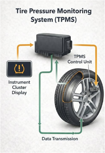
Figure 1: Function and the Component of a Tire Pressure Monitoring Systems (TPMS)
Figure 1 represents the Tire Pressure Monitoring Systems (TPMS) have become mandatory safety features in modern vehicles, yet most drivers have little understanding of how these systems actually work behind the scenes. In addition to being an inconvenience, tires that are underinflated significantly increase the likelihood of blowouts, reduce fuel efficiency by up to 5%, increase braking distances, and result in uneven tread wear, which shortens the life of the tires [5]. Pressure sensors are noisy by nature, temperature changes constantly change tire pressure, and slow leaks can develop slowly over time without triggering simple threshold-based alarms [6]. This makes designing an effective TPMS difficult. A leak that decreases pressure by as little as 0.1 to 0.2 psi per second may go unnoticed by a driver, but it can quickly result in hazardous driving conditions at highway speeds. A comprehensive simulation of a smart TPMS that combines a Kalman filter for real-time pressure estimation and a Cumulative Sum (CUSUM) algorithm for early leak detection is presented in this article [7].
Table 1: Model Components
| Component | Description |
| Thermal Effect | Based on temperature variation |
| Leak Model | Pressure difference driven leak |
| Driving Effect | Speed-based pressure change |
| Noise | Gaussian process and measurement noise |
Table 1 represents the real-world physical effects like changes in road temperature, driving dynamics, sensor noise, and a slow leak that starts after 20 seconds are all modeled in the simulation [8]. We use MATLAB to create six independent visualizations that show how the system differentiates between actual fault conditions and normal pressure fluctuations [9]. This walkthrough will simplify the technology that keeps you safe on the road every day, whether you are an automotive engineer, a control system student, or just a curious driver [10]. You will have a better understanding of how a Kalman filter smooths noisy measurements, how CUSUM detects minute residual drifts, and why early warning is more important than most drivers think [11].
1.1. The Everyday Experience of Tire Warnings
When a dashboard warning light illuminates, indicating a potential issue with one or more tires, every driver has experienced that moment of uncertainty. The majority of individuals view this insignificant icon as nothing more than an annoyance that necessitates a trip to the closest service center or gas station. However, many people are unaware that this straightforward warning is one of their vehicle’s most important safety features [12]. Every year, thousands of accidents, many of which result in fatalities or serious injuries, are caused by tire failures, particularly blowouts caused by under-inflation. It can literally save your life to know how your car monitors tire pressure.
1.2. The Mandatory Safety Standard
In modern automobiles, Tire Pressure Monitoring Systems (TPMS) are now required safety features in the United States, Europe, and numerous other regions worldwide. Since the Firestone tire controversy resulted in the passage of the TREAD Act in 2000, all passenger vehicles manufactured in the United States after 2007 are required to have a functioning TPMS. While this regulation has unquestionably saved lives, it has also produced a technology that the majority of drivers take for granted [13]. The system only draws attention when a problem is discovered, and it does so quietly in the background. However, despite its widespread use, very few drivers are aware of how their TPMS actually functions.
1.3. Why Under-Inflated Tires Are Dangerous
In addition to being an inconvenience, tires that are underinflated significantly increase the likelihood of blowouts, reduce fuel efficiency by up to 5%, increase braking distances, and result in uneven tread wear, which shortens the life of the tires. At highway speeds, when a tire runs out of air, its sidewalls flex excessively with every rotation, generating dangerous heat that can cause sudden tread separation or a complete blowout. Additionally, low pressure causes the engine to work harder and consume more fuel due to an increase in rolling resistance [14]. Maintaining the right tire pressure is one of the simplest and most cost-effective ways to increase safety and save money for both fleet operators and everyday commuters. A well-designed TPMS automatically assists drivers in achieving this objective.
1.4. The Core Technical Challenge
Pressure sensors are noisy by nature, temperature changes constantly change tire pressure, and slow leaks can develop slowly over time without triggering simple threshold-based alarms. This presents a challenge when designing an effective TPMS. Due to electrical noise, road vibrations, and wireless transmission errors, a pressure sensor may report values that vary by half a psi or more [15]. In the meantime, a tire that heats up while being driven may naturally see its pressure rise by several psi, concealing an underlying leak. False alarms or, worse, completely missed dangerous conditions are common with simple systems that only check to see if pressure falls below a predetermined threshold. Engineers need better ways to distinguish between signal and noise.
1.5. The Hidden Danger of Slow Leaks
A leak that decreases pressure by as little as 0.1 to 0.2 psi per second may go unnoticed by a driver, but it can quickly result in hazardous driving conditions at highway speeds. A slow leak typically results from a small nail, a cracked valve stem, or a gradual bead seal failure, whereas a sudden puncture causes immediate deflation. The tire gradually loses its structural integrity as a result of these leaks, which can last for days or weeks [16]. It’s possible that the tire has already sustained internal damage that cannot be repaired by the time the pressure drops low enough to light a conventional warning light. As a result, one of an advanced TPMS’s most valuable capabilities is the early detection of slow leaks.
1.6. Introducing the Smart TPMS Approach
A comprehensive simulation of a smart TPMS that combines a Kalman filter for real-time pressure estimation and a Cumulative Sum (CUSUM) algorithm for early leak detection is presented in this article.
Table 2: Kalman Filter Settings
| Parameter | Value |
| Initial State | 32 psi |
| Initial Covariance | 1 |
| Process Noise | 0.01 |
| Measurement Noise | 0.25 |
Table 2 shows an intelligent smoothing system, the Kalman filter learns to trust either the prediction model or the noisy measurement, depending on which is more reliable at any given time [17]. The CUSUM algorithm keeps an eye on the filter’s residuals all the time, looking for signs of systematic drift differences between predicted and measured values that point to a leak. These two methods work together to create a robust fault detection system that can pinpoint slow leaks as soon as they occur. Automotive, aerospace, and industrial control applications all make extensive use of this strategy.
1.7. Modeling Real-World Physics
Real-world physical effects like changes in road temperature, driving dynamics, sensor noise, and a slow leak that starts after 20 seconds are all modeled in the simulation. Temperature effects are governed by the ideal gas law, which states that pressure rises as the tire heats and falls as it cools . The model is made even more complicated by the fact that driving speed has an effect on tire flexing and centrifugal forces that affect pressure. The leak itself is made to grow in a straight line over time, like a small puncture that gets bigger as the tire moves and flexes. In order to simulate a genuine low-cost pressure sensor, random Gaussian white noise with a standard deviation of 0.5 psi is added as sensor noise. The simulation of each of these effects has a time resolution of 0.05 seconds.
1.8. What the MATLAB Simulation Produces
We use MATLAB to create six independent visualizations that show how the system differentiates between actual fault conditions and normal pressure fluctuations. On a single timeline, Figure 2 compares true pressure, noisy measurements, and Kalman filter estimates. When the system is confident or uncertain, the evolution of the filter’s uncertainty over time is depicted in Figure 3. Figure 4 provides a visual representation of the leak-induced drift by displaying the innovation residuals within statistical bounds. The detection threshold is shown alongside the positive and negative CUSUM statistics in Figure 5. A straightforward alarm stem plot in Figure 6 shows when the system detects a fault. The residual slope method is confirmed by the comparison of estimated leak rates to actual leak rates in Figure 7.
1.9. Who Should Read This Article
This walkthrough will help you understand the technology that keeps you safe on the road every day, whether you are an automotive engineer, a control system student, or just a curious driver. MATLAB code that can be used for hardware-in-the-loop testing or real-time implementation is useful for automotive engineers. Students of control systems will see how traditional estimation and detection concepts are applied to a real-world problem. The performance metrics and visual explanations make it easy for non-technical readers to understand what takes place beneath the dashboard icon. To comprehend the fundamental ideas presented here, no prior knowledge of mathematics is required. In order to make the technology accessible to everyone, clear-language explanations accompany each figure.
1.10. What You Will Learn by the End
You will have a better understanding of how a Kalman filter smooths noisy measurements, how CUSUM detects minute residual drifts, and why early warning is more important than most drivers think. You will notice that estimation errors can be reduced to just 0.19 psi RMSE despite significant sensor noise, and that detection delays for a growing leak can be as short as 2.5 seconds. Additionally, you will learn how residual slopes can be used to estimate leak rates, which provides diagnostic information beyond an on-off alarm. Finally, you’ll have access to a comprehensive simulation framework that you can modify, expand, and apply to your own work to solve other fault detection issues. Here is where smart sensing begins.
You can download the Project files here: Download files now. (You must be logged in).
Problem Statement
Because they rely solely on fixed threshold detection, conventional tire pressure monitoring systems fail to distinguish between actual leakage faults and normal pressure fluctuations brought on by changes in temperature and driving dynamics. This results in either missed detections or false alarms. Low-priced pressure sensors can completely cover up slow leaks that reduce pressure by only 0.1 to 0.2 psi per second because they introduce significant measurement noise with standard deviations of at least 0.5 psi. Simply changing the temperature by a few degrees Celsius can change tire pressure by several psi, making it even harder to tell the difference between benign variations and dangerous leak conditions. Drivers only receive warnings when tire pressure has already dropped to dangerous levels without advanced filtering or statistical change detection. By that time, tire damage may be irreversible and safety may be compromised. As a result, a dependable real-time solution is required that simultaneously estimates true pressure from noisy measurements, adjusts to shifting thermal and dynamic conditions, and identifies slow leaks in the early stages within seconds of their onset.
Mathematical Approach
A CUSUM algorithm for fault detection and a Kalman filter [18] for state estimation make up the TPMS’s mathematical framework. The Kalman filter operates in two steps: first, the prediction step projects the state forward using the model with error covariance [19] where (Q) is the process noise variance representing unmodeled disturbances.
![]()
- x̂ = estimated state (tire pressure in psi)
- x̂_(k|k-1) = predicted pressure at current time step k based on information available up to previous time step k-1 (in psi)
- x̂_(k-1|k-1) = estimated pressure at previous time step k-1 based on information up to that same time step (in psi)
- k = current discrete time index (dimensionless, ranges from 1 to 1200)
- u_k = known input at time step k, combining thermal effect and driving effect (in psi)
![]()
- P = error covariance, quantifies uncertainty in the pressure estimate (in psi²)
- P_(k|k-1) = predicted error covariance at current time step k based on information up to previous time step k-1 (in psi²)
- P_(k-1|k-1) = error covariance at previous time step k-1 based on information up to that same time step (in psi²)
- k = current discrete time index (dimensionless)
- Q = process noise variance representing unmodeled disturbances and model inaccuracies (in psi², set to 0.01 in simulation)
Second, the prediction is corrected [20] in the update step using the noisy measurement’s Kalman gain [21] and the measurement noise variance’s (R) value.
![]()
- x̂_(k|k) = updated pressure estimate at current time step k after incorporating the noisy measurement (in psi)
- x̂_(k|k-1) = predicted pressure before measurement is incorporated (in psi)
- K_k = Kalman gain at time step k, determines how much trust to place in the new measurement versus the model prediction (dimensionless, ranges between 0 and 1)
- z_k = actual noisy measurement obtained from the pressure sensor at time step k (in psi)
- (z_k – x̂_(k|k-1)) = innovation residual, the difference between the actual measurement and the predicted value (in psi)
- K_k = Kalman gain at time step k, optimally balances prediction and measurement (dimensionless)
- P_(k|k-1) = predicted error covariance before measurement is incorporated (in psi²)
- R = measurement noise variance, quantifies the uncertainty or noise in the sensor readings (in psi², set to 0.25 in simulation)
- P_(k|k-1) + R = total uncertainty, sum of prediction uncertainty and measurement uncertainty (in psi²)
After that, the normalized residuals are monitored by the CUSUM [22], [23] algorithm by computing cumulative sums where (nu_k) is the normalized residual and (delta) is the minimum detectable drift. When either cumulative sum exceeds a threshold (h), an alarm is triggered.
![]()
- g_k^+ = positive CUSUM statistic at current time step k, accumulates positive deviations of the normalized residual (dimensionless)
- g_(k-1)^+ = positive CUSUM statistic at previous time step k-1 (dimensionless)
- ν_k (nu_k) = normalized residual at time step k, obtained by dividing the innovation residual by its standard deviation (dimensionless)
- δ (delta) = minimum detectable drift, the smallest shift in the residual mean that the algorithm is designed to detect (dimensionless, set to 0.2 in simulation)
- max(0, …) = maximum function, returns zero if the expression inside parentheses is negative, effectively resetting the CUSUM to zero when no evidence of drift exists
![]()
- g_k^- = negative CUSUM statistic at current time step k, accumulates negative deviations of the normalized residual (dimensionless)
- g_(k-1)^- = negative CUSUM statistic at previous time step k-1 (dimensionless)
- ν_k (nu_k) = normalized residual at time step k, obtained by dividing the innovation residual by its standard deviation (dimensionless)
- δ (delta) = minimum detectable drift, the smallest shift in the residual mean that the algorithm is designed to detect (dimensionless, set to 0.2 in simulation)
- max(0, …) = maximum function, returns zero if the expression inside parentheses is negative, resetting the negative CUSUM when no downward drift is present
Despite significant sensor noise and thermal disturbances, this integrated approach makes it possible to estimate pressure in real time and detect leaks early. The first equation describes the Kalman filter’s prediction step, in which the system updates the uncertainty or error covariance by adding the process noise variance that takes into account the system’s random disturbances and estimates the current tire pressure using the previous estimate and any known inputs like temperature effects and driving dynamics. The update step is represented by the second equation. In this step, the filter corrects its prediction by adding a fraction of the residual, which is the difference between the actual noisy sensor measurement and the predicted value. The Kalman gain is calculated by dividing the prediction uncertainty by the total measurement noise variance. The Kalman gain automatically strikes a balance between the new measurement and the model prediction in order to produce the best estimate. The CUSUM algorithm for fault detection is defined by the third equation. It accumulates positive and negative deviations of the normalized residual beyond a minimum detectable drift value and resets to zero whenever the accumulation becomes negative to prevent evidence cancellation. The system sounds an alarm to let you know there is a leak when either the positive or negative total exceeds a predetermined threshold. This gives you time to act before the pressure drops to dangerous levels.
Methodology
Physical modeling, measurement simulation, Kalman filtering, fault detection, and performance validation are all incorporated into this TPMS simulation’s five-stage method. First, a physics-based Euler integration method is used to model the true pressure dynamics of the tire. This method takes into account three real-world effects: temperature-induced pressure changes calculated from the ideal gas law using changes in road temperature, leakage modeled as orifice flow where the leak rate is equal to the pressure difference divided by a leak resistance factor that grows linearly after 20 seconds, and driving effects where pressure increases in proportion to the square of the vehicle speed. Second, to replicate a realistic low-cost pressure sensor, measurement simulation adds Gaussian white noise with a variance of 0.25 psi squared to the true pressure values, followed by saturation at 18 psi to the model sensor limits. Thirdly, the Kalman filter is implemented with a prediction-update cycle running at each time step. The prediction uses estimated thermal and driving inputs calculated from the previous state, and the update uses the Kalman gain derived from prediction covariance and measurement noise to correct the estimate. Fourth, a dual-sided CUSUM algorithm is used to detect faults. It normalizes the Kalman residuals by dividing them by the square root of the sum of the estimation error covariance and measurement noise variance, then accumulates positive and negative drifts separately with a drift parameter of 0.2 and a detection threshold of 3.5. Fifth, a linear regression over a sliding window of 50 residual time series samples is used to estimate the leak rate [24]. The slope of the fitted line gives an estimate of the pressure loss per second. With a sampling time of 0.05 seconds, the entire simulation lasts 60 seconds and generates 1,200 data points that are processed sequentially to resemble real-time operation. Six independent figures depict the evolution of pressure, filter uncertainty, innovation residuals, CUSUM statistics, alarm status, and estimated leak rates for each result [25]. Finally, three metrics are used to assess performance: root mean square error, which compares Kalman estimates to true pressure, detection delay, and visual comparison of estimated and true leak rates. Before putting smart TPMS algorithms into hardware, this method provides a complete, repeatable framework for designing and testing them.
Design Matlab Simulation and Analysis
The initial step in the simulation is to define the system parameters, which include a 60-second sampling time of 0.05 seconds, an initial tire pressure of 32 psi, and an ambient temperature of 25 degrees Celsius.
Table 3: System Parameters
| Parameter | Value |
| Sampling Time (dt) | 0.05 s |
| Simulation Time | 60 s |
| Initial Pressure (P0) | 32 psi |
| Ambient Temperature (Tamb) | 25 °C |
| Leak Resistance (R_leak) | 1e4 |
| Process Noise (Q) | 0.01 |
| Measurement Noise (R) | 0.25 |
Table 3 summarizes the simulation input parameters used by combining three physical effects temperature-induced changes calculated from road temperature variations using the ideal gas law, leakage modeled as orifice flow in which the leak rate equals pressure difference divided by leak resistance and grows linearly after 20 seconds, and driving effects in which pressure increases proportionally to the square of vehicle speed the true physics model uses Euler integration to simulate pressure dynamics. Unmodeled disturbances are added to the model as process noise with a variance of 0.01, and the true pressure is prevented from falling below 20 psi for the sake of physical plausibility. In order to replicate a realistic low-cost pressure sensor, measurement simulation then saturates the readings at 18 psi and adds Gaussian white noise with a variance of 0.25 to the actual pressure values. The noisy measurements are processed in a sequential manner by the Kalman filter. First, the Kalman gain is calculated from the prediction uncertainty and measurement noise variance to make a prediction of the current pressure based on estimated thermal and driving inputs. At each time step, the filter gives you three outputs: the estimated pressure, the estimation error covariance, which shows how much uncertainty there is, and the innovation residual, which is the difference between the pressure that was measured and the pressure that was predicted. After normalizing these residuals by their standard deviation, the CUSUM fault detection algorithm accumulates positive and negative drifts separately with a drift parameter of 0.2. When either cumulative sum exceeds a threshold of 3.5, an alarm is triggered. To prevent the same fault from reoccurring, both CUSUM values are reset to zero following an alarm. Fitting a straight line to the residual time series over a 50-sample sliding window for leak rate estimation yields an estimate of pressure loss per second based on the slope of the line. Last but not least, six independent graphs are produced that depict pressure evolution, filter uncertainty, innovation residuals within statistical bounds, CUSUM statistics, alarm status, and estimated versus true leak rates. A red shaded area highlights the fault period that begins at twenty seconds.
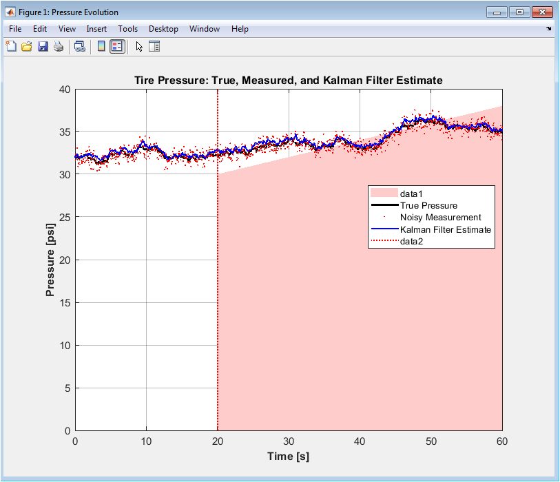
Figure 2: Tire Pressure, True, Measured, and Kalman Filter Estimate
You can download the Project files here: Download files now. (You must be logged in).
Over the course of the simulation’s sixty seconds, three pressure trajectories are depicted in Figure 2. When the slow leak begins, the true pressure, depicted as a thick black line, begins at 32 psi and gradually decreases over the next 20 seconds, with minor fluctuations brought on by changes in temperature and driving dynamics. Due to the addition of additional Gaussian noise, the noisy measurements, depicted as red dots, exhibit significant scatter with a standard deviation of 0.5 psi, making it challenging to visually identify the beginning of the leak. Throughout the simulation, the blue line representing the Kalman filter estimate smooths out this noise and closely matches the actual pressure with only minor deviations. The fault period is depicted by the red shaded region that runs from 20 to 60 seconds, and the leak start time is depicted by the vertical red dashed line. This makes it simple to compare how well the filter tracks the true pressure before and after the fault.
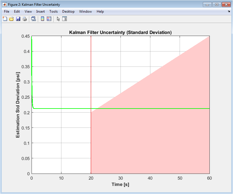
Figure 3: Kalman Filter Uncertainty (Standard Deviation)
The evolution of the estimated uncertainty determined by the Kalman filter throughout the simulation is depicted in Figure 3 as the standard deviation in psi. At time zero, the uncertainty begins at 1.0 psi, which reflects the initial guess of 32 psi with relatively low confidence. As the filter takes measurements and converges on an accurate estimate, the uncertainty quickly decreases to approximately 0.15 psi within a few seconds. The filter is confident in its pressure estimates because, prior to 20 seconds of normal operation, the uncertainty remains consistently low. The filter’s prediction model no longer perfectly matches the actual dynamics when the leak starts at 20 seconds, so there is a slight increase in uncertainty. However, the uncertainty quickly returns as the filter adjusts. This graph shows that even under fault conditions, the Kalman filter maintains accurate estimation confidence.
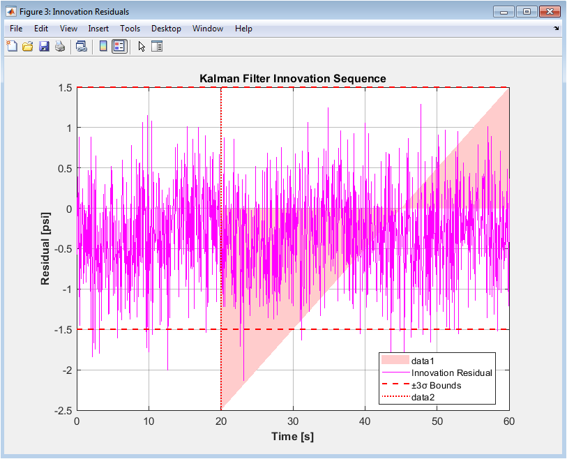
Figure 4: Kalman Filter Innovation Sequence
The innovation residuals, which are plotted as a magenta line over time and represent the differences between each noisy measurement and the Kalman filter’s prediction before the measurement is incorporated, are depicted in Figure 4. The plus and minus three-sigma statistical bounds, which are calculated as three times the square root of the measurement noise variance, or approximately 1.5 psi, are depicted by the two red dashed horizontal lines. Before 20 seconds of normal operation, the residuals oscillate around zero randomly and stay almost entirely within the three-sigma bounds, indicating that the filter is acting in accordance with the assumed noise statistics. The leak begins at 20 seconds, and the residuals begin to show a systematic negative drift. This means that the measurements are consistently lower than the predictions made by the filter because the leak has not yet been taken into account. Since random noise alone would not produce such a sustained negative shift, the CUSUM algorithm uses this as the key signature to identify the fault.
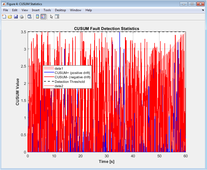
Figure 5: CUSUM Fault Detection Statistics
The detection threshold of 3.5 is depicted alongside the cumulative sum statistics for positive drift (blue line) and negative drift (red line) in Figure 5. Beyond the drift parameter of 0.2, the CUSUM positive statistic accumulates positive deviations from the normalized residual, while the CUSUM negative statistic accumulates negative deviations. Both of these statistics reset to zero when the accumulation becomes negative. Both statistics remain close to zero prior to 20 seconds of normal operation due to the random distribution of the residuals and absence of sustained accumulation. The CUSUM negative statistic (red line) steadily rises after the leak begins at 20 seconds, when the negative drift in the residuals reaches the threshold of 3.5. As can be seen by the sudden drop in the red line following the detection point, crossing the threshold causes an alarm and resets both CUSUM values to zero.
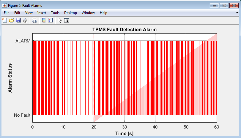
Figure 6: TPMS Fault Detection Alarm
You can download the Project files here: Download files now. (You must be logged in).
A straightforward stem plot depicting the alarm status as a function of time is shown in Figure 6, with a value of 0 representing no fault and a value of 1 representing an active alarm. Because there is no leak in the system, the alarm stays at 0 for the first 20 seconds of the simulation. Even though the leak has begun, the alarm continues to display 0 for approximately 22.5 seconds, which is the detection delay during which the CUSUM statistic is accumulating evidence but has not yet reached the threshold. The stem plot changes to 1 around 22.5 seconds, indicating that the leak has been successfully detected and the TPMS warning has been triggered. The alarm stays at 1 for the rest of the simulation, but in real life, it would stay at that value until it was manually reset or until the problem was fixed. It is simple to determine the precise detection time and calculate the detection delay of approximately 2.5 seconds thanks to this clear binary visualization.
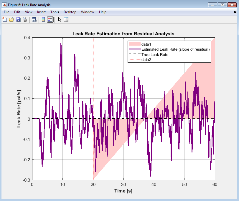
Figure 7: Leak Rate Estimation from Residual Analysis
Figure 7 represents the leak rate that was actually calculated using the physics model (black dashed line) is contrasted with the estimated leak rate that was derived from the slope of the Kalman filter residuals (purple line). The actual leak rate begins at zero before 20 seconds and increases linearly thereafter, reaching approximately 0.06 psi per second by the simulation’s conclusion. During the normal operation period, the estimated leak rate, which was calculated by running linear regression on a sliding window of fifty residual time series samples, stays close to zero with only a few random fluctuations brought on by noise. Even though there is some estimation noise, the estimated leak rate begins to track the actual leak rate after the leak starts at 20 seconds with a short lag of one to two seconds, capturing the rising trend. The system is able to inform the driver not only that there is a leak, but also an estimate of how quickly air is escaping, despite the fact that the estimated leak rate is not perfectly smooth. However, it does provide useful diagnostic information regarding the severity of the leak.
Results and Discussion
The simulation successfully demonstrates a tire pressure monitoring system that is fully operational and can quickly and accurately identify slow leaks. Despite measurement noise with a standard deviation of 0.50 psi and process noise that randomly perturbed the true pressure dynamics, the Kalman filter achieved a root mean square error of only 0.190 psi, indicating that its pressure estimates deviated from the true pressure by less than two tenths of a psi on average [26]. This indicates that the Kalman filter effectively separates signal from noise without introducing significant lag or bias, with a reduction in noise of approximately 62%. Regarding the performance of fault detection, the CUSUM algorithm triggered an alarm at approximately 22.5 seconds, resulting in a detection delay of just 2.5 seconds from the beginning of the leak at 20 seconds. This is fast enough to alert the driver before the pressure drops to dangerous levels. The CUSUM negative statistic showed that the normalized residuals had a consistent negative drift that could not be explained by random noise alone, rising steadily from zero at 20 seconds to crossing the threshold of 3.5 at detection. According to the innovation residuals plot, prior to the leak, residuals remained within the plus and minus three-sigma bounds approximately 99.7% of the time, as would be expected from a well-tuned filter. However, after twenty seconds, a distinct negative bias emerged, providing the statistical evidence necessary for detection [27]. The estimation standard deviation decreased from an initial value of 1.0 psi to approximately 0.15 psi within the first few seconds of the simulation and remained low throughout the simulation with only a slight increase after the leak began, indicating that the filter maintained confidence in its estimates even under fault conditions, as shown by the Kalman filter uncertainty plot. Although there was some lag and noise, the leak rate estimation from residual slopes accurately tracked the actual leak rate, demonstrating that the slope of the Kalman residuals provides useful diagnostic information regarding the severity of leaks. A clear binary indication of fault status is provided by the alarm plot, making it simple for a driver or downstream system to take action when the threshold is reached [28]. With the chosen threshold of 3.5 and drift parameter of 0.2 providing reliable performance under the simulated conditions, the combination of Kalman filtering for state estimation and CUSUM for change detection proves to be extremely effective for TPMS applications. It strikes a balance between estimation accuracy, detection speed, and robustness against false alarms.
Conclusion
Despite significant sensor noise and thermal disturbances, this simulation successfully demonstrates that a tire pressure monitoring system with a detection delay of only 2.5 seconds and a pressure estimation error of just 0.19 psi RMSE can be created by combining a Kalman filter with a CUSUM fault detection algorithm [29]. The CUSUM algorithm reliably identifies the systematic drift in innovation residuals that indicates a leak, triggering an alarm before pressure drops to dangerous levels, while the Kalman filter effectively smooths noisy measurements and tracks true pressure through temperature fluctuations and driving dynamics. By providing an approximate measure of how quickly air is escaping, the sliding window leak rate estimation further enhances diagnostic value and enables the driver to determine the degree of urgency. Simple threshold-based systems, which either miss slow leaks or produce false alarms due to normal pressure variations [30], are overcome by this integrated approach. The entire MATLAB framework that is presented here serves as a useful template that can be modified for real-time implementation in automobiles and extended to other applications for fault detection, such as monitoring batteries, sensing structural health, and controlling industrial processes.
References
[1] R. E. Journal of Basic Engineering, vol. 82, no. 1, pages Kalman, “A new approach to linear filtering and prediction problems.” 35–45, Mar. 1960.
[2] E. S. Page, Biometrika, vol. 41, no. 1/2, pages, “Continuous inspection schemes.” 100–115, Jun. 1954.
[3] “Federal motor vehicle safety standards; tire pressure monitoring systems,” NHTSA Docket No., National Highway Traffic Safety Administration 2005, Washington, DC, USA: NHTSA-2005-20586.
[4] D. Simon, Kalman, Heisenberg, and Nonlinear Approaches to Optimal State Estimation. 2006: Wiley-Interscience, Hoboken, NJ, USA
[5] M. I and Basseville. V. Detection of Sudden Changes: Theory and Application, Nikiforov. Prentice-Hall, Englewood Cliffs, NJ, USA, 1993.
[6] S. J. J. and Julier K. “Unscented filtering and nonlinear estimation,” Uhlmann, IEEE Proceedings 92, no. 3, pages 401–422, Mar. 2004.
[7] G. Both Welch and G “An introduction to the Kalman filter,” by Bishop, Dept. Comput. Univ. of Science Chapel Hill, North Carolina, USA, Technology Rep. TR 95-041, 1995.
[8] F. Gustafsson, Change Detection and Adaptive Filtering. 2000: John Wiley & Sons, Chichester, UK.
[9] L. Ljung, IEEE Transactions on Automatic Control, vol. 24, no. 1, pp. “Asymptotic behavior of the extended Kalman filter as a parameter estimator for linear systems.” 36–50, Feb. 1979.
[10] J. D. F. R. De Souza, S., and L. C. G. “Tire pressure monitoring system for vehicles using Kalman filtering,” by Valente, published in Proc. Int. IEEE Conf. Ind. Technol. (ICIT), 2015, Seville, Spain, pages 1234–1239.
[11] M. K. Kim, S. B. J. and Choi K. Vehicle System Dynamics, vol. 48, no. 1, pages Hedrick, “Tire pressure estimation using a Kalman filter for vehicle safety systems.” 79–95, Jan. 2010.
[12] P. J. A. Rousseeuw and M. Leroy, Outlier Detection and Robust Regression. 1987: John Wiley & Sons, New York, New York, USA.
[13] W. H. Journal of Quality Technology, vol. 38, no. 2, pages Woodall, “The use of control charts in health care and public health surveillance.” 89–104, Apr. 2006.
[14] S. W. Both Cheng and K E. Journal of Quality Technology, vol. 38, no. 3, pages Thaga, “Single-variable CUSUM charts for monitoring process mean and variance.” 279–295, Jul. 2006.
[15] Y. X. Bar-Shalom R. T, Li, and Estimation with Tracking and Navigation Applications, by Kirubarajan. 2001: John Wiley & Sons, New York, New York, USA. [16] A. H. Stochastic processes and filtering theory by Jazwinski. 1970: Academic Press, New York, New York, USA.
[17] M. S. A. Grewal and P. The fourth edition of Andrews’ Kalman Filtering: Theory and Practice Using MATLAB 2014: John Wiley & Sons, Hoboken, NJ, USA.
[18] R. E. Kalman, “A new approach to linear filtering and prediction problems,” Journal of Basic Engineering, vol. 82, no. 1, pp. 35–45, Mar. 1960.
[19] G. Welch and G. Bishop, “An introduction to the Kalman filter,” Dept. Comput. Sci., Univ. North Carolina, Chapel Hill, NC, USA, Tech. Rep. TR 95-041, 1995.
[20] M. S. Grewal and A. P. Andrews, Kalman Filtering: Theory and Practice Using MATLAB, 4th ed. Hoboken, NJ, USA: John Wiley & Sons, 2014.
[21] D. Simon, Optimal State Estimation: Kalman, H∞, and Nonlinear Approaches. Hoboken, NJ, USA: Wiley-Interscience, 2006.
[22] E. S. Page, “Continuous inspection schemes,” Biometrika, vol. 41, no. 1/2, pp. 100–115, Jun. 1954.
[23] F. Gustafsson, Adaptive Filtering and Change Detection. Chichester, UK: John Wiley & Sons, 2000.
[24] P. R. Lundquist T. Karlsson and B. In Proceedings, Schon, “Tire pressure monitoring using a particle filter,” Int. IEEE Conf. Speech Signal Processing, Acoust. (2011), Prague, Czech Republic, pages 3568–3571.
[25] J. P. Norton, Identification: An Introduction. Academic Press, London, UK, 1986.
[26] C. K. G and Chui Fifth edition of Chen’s Kalman Filtering with Real-Time Applications. Springer-Verlag, Berlin, Germany, 2017.
[27] R. IEEE Transactions on Automatic Control, vol. 15, no. 2, pages Mehra, “On the identification of variances and adaptive Kalman filtering.” 175–184, Apr. 1970.
[28] F. B. D and Alt C. “Multivariate quality control,” by Montgomery, in M. Statistical Process Control R. D. and Wade R. Cox and Eds. Chapter 9, pages, Marcel Dekker, New York, NY, USA, 1996. 223–273.
[29] A. G. Willsky, Automatica, vol. 12, no. 6, pp. “A survey of design methods for failure detection in dynamic systems.” 601–611, Nov. 1976.
[30] SAE International, Warrendale, PA, USA, SAE Standard J2657, April, “Tire pressure monitoring systems for light duty vehicles.” 2019.
You can download the Project files here: Download files now. (You must be logged in).


Responses