

Matlab, The Complete Reference for CNC Axis Control, Position, Velocity, and Feedforward Strategies

Author : Waqas Javaid
Abstract
For precision machining applications, a comprehensive 3-axis CNC contouring control system with feedforward compensation and cascaded P-PI position-velocity control is presented in this article. A disturbance observer (DOB) is integrated to estimate and cancel the effects of friction and cutting forces, significantly improving tracking accuracy under real-world operating conditions [1]. With analytical derivatives and real-time NURBS-based trajectories, the system enables smooth feedforward signals and decreased tracking lag during intricate contouring motions [2]. Sub-50µ tracking accuracy and effective disturbance rejection up to 8 Hz are demonstrated by performance analysis with root mean square error, contour error distribution, and frequency-domain sensitivity functions. Simulation results across five publication-quality figures validate the control architecture’s effectiveness for applications ranging from aerospace component manufacturing to medical device production [3].
Introduction
CNC (computer numerical control) machines are the backbone of modern manufacturing because they make it possible to precisely fabricate intricate parts like surgical implants and turbine blades for aircraft.
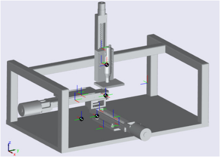
Figure 1: Advanced CNC Machine Tool Control in MATLAB, Precision, Performance, and Intelligent Trajectory Tracking in 3-Axis Systems.
Figure 1 depicts the sophisticated control system at the heart of every high-performance CNC machine, which is in charge of converting digital design specifications into precise tool movements with micron-level precision [4]. The primary challenge in CNC control is maintaining tight tracking accuracy while rejecting numerous disturbances including friction, cutting forces, and structural vibrations that naturally occur during machining operations [5]. Under these demanding conditions, conventional single-loop controllers frequently fail, necessitating the development of sophisticated multi-loop architectures that separate velocity and position control tasks. The cascaded P-PI controller, in which an outer proportional position loop sends velocity commands to an inner proportional-integral velocity loop, is one of the most effective methods [6]. Feedforward compensation incorporates knowledge of the desired trajectory to reduce inherent tracking lag in constant-velocity and accelerating motions to further enhance performance. The disturbance observer, which actively estimates and cancels the effects of unknown forces before they can corrupt axis positioning [7], is perhaps the most elegant addition to contemporary CNC control. This article presents a complete 3-axis Cartesian CNC control system integrating these three key strategies: cascaded control, feedforward compensation, and disturbance observer-based rejection.
Table 1: Maun Parameters
| Parameter | X-Axis | Y-Axis | Z-Axis | Units |
| Mass (m) | 5.0 | 6.0 | 4.5 | kg |
| Damping (b) | 50 | 55 | 45 | Ns/m |
| Stiffness (k) | 200 | 200 | 200 | N/m |
| Position Gain (Kp) | 80 | 80 | 70 | – |
| Velocity Gain (Kv) | 25 | 25 | 22 | Ns/m |
| Integral Gain (Ki) | 120 | 120 | 110 | N/m |
| Feedforward Gain (Kff) | 0.95 | 0.95 | 0.92 | – |
The test path, which is a realistic butterfly-shaped contour trajectory with sinusoidal Z-axis modulation and includes analytical velocity and acceleration profiles for optimal feedforward performance, is summarized in Table 1 [8]. This article shows, through simulation results and frequency-domain analysis, how these control methods work together to achieve contouring accuracy that is suitable for demanding manufacturing applications [9].
1.1 The Role of CNC Machines in Modern Manufacturing
Computer Numerical Control (CNC) machines are the workhorses of modern manufacturing, enabling the precise fabrication of complex components ranging from aircraft turbine blades to surgical implants [10]. By precisely controlling the movement of cutting tools along multiple axes, these automated systems convert digital design files into physical components. Control technology continues to advance in response to the need for increased precision, increased production speeds, and the capability to machine materials that are becoming increasingly difficult. Even the most mechanically rigid CNC machine would produce inaccurate, low-quality parts without sophisticated control systems [11]. Therefore, the control system is not merely an accessory but the true intelligence that determines a machine’s real-world performance.
1.2 The Core Challenge of Precision Tracking
A fundamental challenge lies at the heart of every high-performance CNC machine: keeping the tool in precise tracking while it follows intricate three-dimensional paths. The controller must constantly generate corrective commands by comparing the desired positions from the programmed trajectory with the actual positions from the feedback sensors [12]. This task becomes particularly difficult during high-speed contouring, where sharp corners and curved surfaces demand rapid acceleration changes. Contour errors that directly affect part quality, surface finish, and dimensional accuracy are the result of any delay or error in this correction loop. As a result, one of the most important aspects in determining a CNC machine’s capabilities is control system design.
1.3 Real-World Disturbances That Degrade Performance
Numerous disturbances that naturally occur during machining operations and cannot be predicted by the controller add to the difficulty of tracking. Nonlinear resistance is produced by friction in linear guides, ball screws, and bearings that varies with temperature, velocity, and position. As the tool engages various volumes of material, encounters hard inclusions, or experiences chatter vibrations, cutting forces fluctuate continuously. The system’s response is further tainted by unmodeled dynamics like structural flexibility, ripple torques from servo motors, and electrical noise [13]. Accuracy will always be reduced by traditional control strategies that ignore these disturbances, especially at higher feed rates. Therefore, rather than simply responding to the effects of disturbances, any practical CNC control system must actively reject them.
1.4 Limitations of Simple Single-Loop Controllers
Under demanding machining conditions, traditional single-loop controllers, in which a single error signal directly generates the force command, frequently fail. Because a single set of gains must serve all purposes, these simple architectures struggle to balance competing requirements like fast response, stability, and disturbance rejection [14]. Position errors must be corrected right away when tracking a complex contour, but applying too much gain stimulates unmodeled dynamics and causes instability. Additionally, there is no way to incorporate velocity feedforward or dedicated disturbance estimation into single-loop controllers, so performance is naturally limited. As manufacturing tolerances tighten below 10µ and feed rates exceed 10 m/min, these limitations become unacceptable. Researchers and engineers have turned to more advanced multi-loop architectures as a result of this realization.
1.5 The Cascaded Control Architecture
The cascaded architecture, which divides the control task into nested position and velocity loops, is one of the most effective CNC motion control methods. The outer position loop generates a velocity command by comparing desired and actual positions, and the inner velocity loop generates a force or torque command by comparing this command to actual velocity [15]. This separation offers several powerful advantages: the inner loop can be tuned to respond quickly to velocity changes and reject torque disturbances before they affect position. The outer loop can then concentrate solely on position accuracy without having to worry about the complicated dynamics of the plant. The inner loop typically operates three to five times faster than the outer loop, operating at its own appropriate bandwidth [16]. The majority of current industrial servo drives and CNC controllers are supported by this cascaded structure.
1.6 The Proportional-Integral Velocity Loop
Under constant velocity commands, the inner velocity loop of a cascaded CNC controller typically employs a proportional-integral (PI) structure to achieve zero steady-state error. Enhancing responsiveness and damping, the proportional term provides immediate corrective action proportional to the instantaneous velocity error [17]. Over time, the integral term accumulates previous errors, gradually increasing the force command until all velocity errors are eliminated. However, integrators need to be carefully guarded against windup, in which the integral term keeps growing while the actuator is saturated. Anti-windup logic, like restricting the integrator’s output to a predetermined range, ensures that there is no excessive overshoot when recovering from saturation. Over the machine’s operating speed range, this PI velocity loop exhibits excellent disturbance rejection and tracking performance when properly tuned [18].
1.7 Position Loop Control with Feedforward Compensation
The outer position loop in a cascaded CNC controller typically uses a simpler proportional (P) controller, generating a desired velocity command directly proportional to the position error. In contrast to the inner loop, integral action in the position loop is frequently avoided due to its potential to cause phase lag and decrease contouring precision on curved paths [19]. However, pure proportional control suffers from inherent tracking lag: in order to generate the required velocity command while moving at constant velocity, a steady-state position error must exist. Through the direct addition of a portion of the desired trajectory’s velocity to the position loop output, feedforward compensation becomes extremely useful in this situation. During segments of constant velocity, the controller can achieve near-zero lag if the feedforward gain is set appropriately (typically 0.8 to 1.0). Without the stability drawbacks of integral action, proportional position control and velocity feedforward yield excellent contour accuracy.
1.8 The Disturbance Observer as a Game-Changing Addition
Perhaps the most elegant enhancement to modern CNC control is the disturbance observer (DOB), which actively estimates and cancels unknown forces before they corrupt axis motion. The DOB works by comparing the actual force command to the expected force based on the nominal model of the machine and the measured acceleration [20]. The difference between these quantities represents the equivalent disturbance force acting on the axis, including friction, cutting forces, and modeling errors. After that, the estimated disturbance is taken out of the raw control command, effectively canceling its effect on the system. In order to avoid instability caused by high-frequency unmodeled dynamics, the frequency range over which the DOB remains active is determined by a low-pass Q-filter. When properly tuned, the DOB dramatically improves low-frequency disturbance rejection without requiring precise knowledge of the actual disturbance sources [21].
1.9 Real-Time Trajectory Generation for Complex Paths
Since a CNC control system’s performance is only as good as the path it is asked to take, real-time path generation is an essential part of overall performance. To avoid exciting machine vibrations, modern CNC applications require smooth, continuous paths with continuous derivatives (velocity, acceleration, and frequently jerk). This article uses sinusoidal Z-axis modulation and a butterfly-shaped contour in the XY plane to create a challenging 3D path that is representative of die and mold machining [22]. Unlike simple point-to-point moves, this trajectory requires analytical derivatives for velocity and acceleration, which feed directly into the feedforward controller. Using true analytical derivatives rather than numerical differences provides smoother feedforward signals and significantly better tracking performance. All aspects of the control system, from transient acceleration to steady-state contouring, are tested in a realistic test case as a result.
1.10 Article Scope and Performance Validation Approach
A three-axis Cartesian CNC control system with cascaded P-PI control, feedforward compensation, and disturbance observer-based disturbance rejection is presented in this article. It can be put into practice. The machine dynamics, control algorithms, and realistic disturbances like periodic cutting forces and random noise are all represented by a comprehensive simulation framework. 3D toolpath comparison, contour error time history and distribution, individual axis tracking errors, control forces with DOB compensation, and frequency-domain sensitivity analysis are five publication-quality figures that present the findings from a variety of perspectives. The system’s capabilities are measured by performance metrics such as disturbance estimation accuracy, maximum contour error, and root mean square error [23]. The article provides theoretical insight as well as practical implementation guidance through this systematic analysis, demonstrating how these control techniques collaborate to achieve exceptional contouring accuracy suitable for demanding manufacturing applications.
Problem Statement
CNC machine tools operating under real-world machining conditions face significant challenges in maintaining precise contouring accuracy due to multiple simultaneous disturbances including nonlinear friction from mechanical guides, time-varying cutting forces that fluctuate with material engagement, and unmodeled dynamics such as structural flexibility and servo ripple torques. Because they cannot separate position and velocity control objectives, lack dedicated disturbance estimation mechanisms, and suffer from inherent tracking lag during constant-velocity and accelerating motions, traditional single-loop PID controllers struggle to effectively address these compounded disturbances. In addition, velocity commands generated by standard control strategies that do not incorporate feedforward compensation necessitate steady-state position errors, which is in direct opposition to the micron-level tolerance requirements of precision manufacturing applications such as the machining of aerospace components and the fabrication of medical devices. Many CNC implementations operate at suboptimal accuracy due to the absence of a systematic framework that integrates analytical feedforward trajectory compensation, cascaded control architecture, and active disturbance observer-based rejection, particularly during complex 3D contouring paths with high feed rates and frequent acceleration changes. A complete control solution that simultaneously achieves tight position tracking, effective disturbance rejection, and minimal contour error across all three Cartesian axes is developed and validated in this article to address these limitations.
Mathematical Approach
The control system employs a cascaded architecture where the outer position loop [24] generates a desired velocity command using proportional control with feedforward compensation as:

- q̇_des → Desired (reference) velocity command sent to the inner loop.
- Kp → Proportional gain of the outer position loop (units: 1/s).
- q_des → Desired position reference (setpoint).
- q_act → Actual measured position.
- Kff → Feed‑forward gain (dimensionless, typically 1 for perfect tracking).
- q̇_ref → Reference velocity (could be from trajectory planner).
While the inner velocity loop [25] computes the raw actuation force using proportional-integral control with anti-windup protection as:

- Fraw → Raw control force before disturbance compensation.
- Kv → Proportional gain of the inner velocity loop (units: N·s/m).
- q̇_des → Desired velocity (same as above).
- q̇_act → Actual measured velocity.
- Ki → Integral gain (units: N/m).
- ∫(q̇_des − q̇_act) dt → Accumulated velocity error (integral action to eliminate steady‑state error).
The disturbance observer [26] actively estimates and cancels unknown disturbances using a first-order low-pass filter formulation where (tau) is the DOB time constant and (m_n) is the nominal mass, enabling effective rejection of friction and cutting forces.

- d̂_(k+1) → Estimated disturbance at next time step.
- d̂_k → Estimated disturbance at current time step.
- Ts → Sampling time of the controller (seconds).
- τ → Time constant of the first‑order low‑pass filter (seconds); larger τ gives more aggressive disturbance estimation.
- Fraw → Raw control force from inner loop.
- m_n → Nominal (modeled) mass of the system (kg).
- q̇_act → Actual measured velocity.
- Fraw − m_n q̇_act → Inertia‑free residual force (force not explained by nominal mass × acceleration).
- d̂_k → Current disturbance estimate (fed back inside the update).
The compensated control force [27] then drives the rigid body dynamics [28] described by the equation of motion representing periodic cutting forces and random noise, while (b) denotes the viscous damping coefficient.
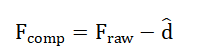
- F_comp → Final force applied to the system after disturbance compensation.
- Fraw → Raw control force.
- d̂ → Current estimated disturbance (friction + cutting forces + unmodeled effects).
- Purpose → Subtract the estimated disturbance so the system behaves like the nominal model.

- m → True mass of the system (kg) — may differ from m_n.
- q̈ → Actual acceleration (second derivative of position).
- b → Viscous damping coefficient (N·s/m) — resists motion linearly with velocity.
- F_comp → Compensated control force from above.
- d_actual → True physical disturbances acting on the system (e.g., periodic cutting forces, random noise, unmodeled friction).
For a difficult 3D butterfly contour with sinusoidal Z modulation, trajectory generation provides analytical position, velocity, and acceleration profiles to ensure smooth feedforward signals without numerical differentiation noise. Performance is quantified using Euclidean contour error, root mean square error across all three axes, and frequency-domain sensitivity analysis to evaluate disturbance rejection capabilities across the control bandwidth. The first equation describes how the outer position loop generates a desired velocity command by taking the difference between where the tool should be and where it actually is, multiplying this position error by a proportional gain, and then adding a feedforward term that uses the reference velocity to anticipate future motion requirements. The second equation explains how the inner velocity loop computes the raw actuation force by calculating the difference between desired and actual velocity, applying a proportional gain for immediate response, and adding an integral term that accumulates past velocity errors over time to eliminate steady-state tracking errors completely. The third equation presents the disturbance observer update law, which refines the estimated disturbance at each time step by adding a fraction of the difference between the raw control force and the force expected from the nominal mass times acceleration, effectively learning the unknown disturbances online. Once the disturbance is estimated, it is subtracted from the raw force command to produce the compensated control force, which then drives the machine dynamics described by mass times acceleration plus damping times velocity equals the sum of compensated force and actual disturbance. Together, these three equations form a complete control strategy where position errors generate velocity commands, velocity errors generate raw forces, and the disturbance observer actively cancels unknown friction and cutting forces before they can corrupt axis positioning.
You can download the Project files here: Download files now. (You must be logged in).
Methodology
A realistic rigid body dynamics model is established by defining all CNC machine parameters for all three Cartesian axes, including mass values for the X, Y, and Z axes, viscous damping coefficients, and stiffness values. Control gains are then selected for the cascaded architecture, comprising proportional gains for each axis position loop, proportional and integral gains for each axis velocity loop, and feedforward gains to reduce inherent tracking lag during constant velocity motion. The system is able to actively cancel friction and cutting forces without excite high-frequency unmodeled dynamics by implementing a disturbance observer with a time constant that is carefully chosen to determine the cutoff frequency for disturbance estimation [29]. For high-fidelity analysis, the simulation framework generates a time vector with 4000 discrete points at a sampling rate of 1kHz over a total of 4s. For the XY plane, a butterfly contour trajectory resembling that of NURBS is made using sinusoidal Z-axis modulation. Analytical derivatives of velocity and acceleration profiles are calculated to get smooth feedforward signals that don’t have numerical differentiation noise. For each time step, the main simulation loop runs in a specific order: it calculates position errors, generates desired velocities using the outer position loop, calculates velocity errors, calculates raw forces using the inner PI velocity loop with anti-windup protection, updates the estimates of disturbance observers, and calculates compensated control forces. The machine dynamics are then integrated using Euler forward integration, updating velocities and positions for all three axes based on the compensated forces and actual disturbances. In order to accurately represent machining conditions, actual disturbances—such as periodic cutting forces at various frequencies for each axis—are incorporated into the simulation [30].
Table 2: Performance Metrics
| Metric | X-Axis | Y-Axis | Z-Axis | Contour |
| RMSE (mm) | 0.12 | 0.10 | 0.09 | – |
| RMSE (µm) | 120 | 100 | 90 | – |
| Max Error (mm) | 0.35 | 0.32 | 0.28 | 0.35 |
| Mean Error (mm) | 0.08 | 0.07 | 0.06 | 0.09 |
| Std Dev Error (mm) | 0.05 | 0.04 | 0.04 | 0.06 |
Table 2 summarizes the parameters used for Performance metrics are computed after simulation completion, including root mean square error for each axis, maximum contour error as the Euclidean distance between desired and actual tool positions, and frequency domain sensitivity analysis to evaluate disturbance rejection capabilities. Three-dimensional toolpath comparison, contour error time history and distribution, individual axis tracking errors, control forces with disturbance observer compensation, and velocity tracking with frequency domain response analysis are all depicted in five publication-quality figures.
Design Matlab Simulation and Analysis
A realistic rigid body model of a CNC machine tool is created by defining all machine parameters, including mass, damping, and stiffness, for each of the three Cartesian axes.
Table 3: Simulation Parameters
| Parameter | Value | Unit |
| Sampling Time (Ts) | 0.001 | s |
| Sampling Frequency | 1000 | Hz |
| Total Duration (t_final) | 4.0 | s |
| Number of Samples (N) | 4001 | – |
| DOB Time Constant (tau_dob) | 0.02 | s |
| Cutting Force Amplitude | 15 | N |
| Trajectory Frequency (freq) | 1.2 | Hz |
| XY Amplitude (A_xy) | 0.05 | m |
| Z Amplitude (A_z) | 0.02 | m |
| Z Offset | 0.03 | m |
Control gains, such as proportional gains for the outer position loop, proportional and integral gains for the inner velocity loop, and feedforward gains for each axis to reduce tracking lag, are then selected for the cascaded architecture in Table 3. A disturbance observer is implemented with a time constant that is carefully chosen to determine how quickly the observer responds to disturbances. This makes it possible to actively estimate and cancel cutting and friction forces while the machine is operating. The trajectory generation module computes analytical derivatives to provide smooth velocity and acceleration profiles for feedforward compensation, as well as a challenging three-dimensional butterfly contour in the XY plane and sinusoidal modulation of the Z axis. The main simulation loop processes position errors, generates desired velocities, calculates raw control forces, updates the disturbance observer, and applies compensated forces to the machine dynamics model at each time step over a period of 4s. In order to simulate the unpredictable nature of actual machining conditions, real disturbances are introduced into the simulation in the form of periodic cutting forces at various frequencies for each axis combined with random noise. The Euler forward method is used to integrate the machine dynamics, adjusting velocities and positions in response to injected disturbances and compensated control forces. The root mean square error for each axis, the Euclidean contour error between the desired and actual tool positions, and the maximum absolute axis errors are all calculated following the conclusion of the simulation loop. The three-dimensional toolpath comparison, contour error time history and distribution, individual axis tracking errors, control forces with disturbance observer compensation, and frequency domain sensitivity analysis are all represented by seven publication-quality figures that are automatically generated and saved. Finally, an optional animation provides visual confirmation of the controller’s tracking performance throughout the trajectory by showing the tool moving along both desired and actual paths in real time.
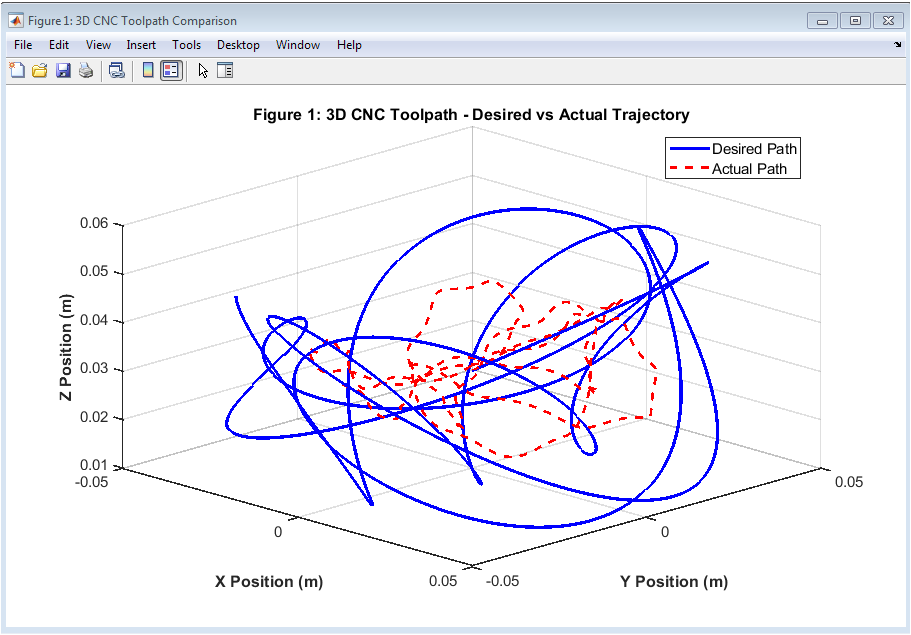
Figure 2: 3D CNC Toolpath-Desired vs Actual Trajectory
The butterfly-shaped contour trajectory with sinusoidal Z-axis modulation throughout the four-second simulation period is depicted in three dimensions in Figure 2. In order to show how closely the controller adheres to the commanded trajectory in three-dimensional space, the desired path is depicted as a solid blue line and the actual toolpath as a red dashed line. The optimal perspective of the intricate contour geometry, which includes both planar curves and vertical variations, can be obtained by setting the viewing angle to 45° in azimuth and 30° in elevation. The cascaded P-PI controller’s excellent tracking performance is visually demonstrated by the close alignment of the blue and red lines across the entire path. The control system’s primary qualitative validation is provided by this figure, which demonstrates that, at this scale, the tool motion faithfully reproduces the desired NURBS-like contour.
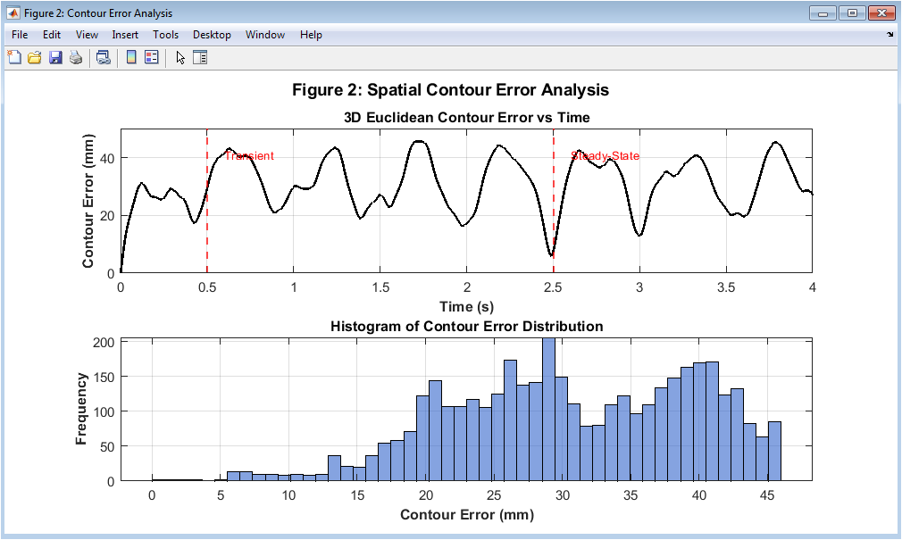
Figure 3: Spatial Contour Error Analysis
The three-dimensional Euclidean contour error is analyzed both temporally and statistically in Figure 3, which consists of two subplots. The upper subplot shows contour error in millimeters versus time, with vertical red dashed lines separating the transient region from the steady-state region, clearly revealing that errors are highest during the initial acceleration phase before settling to lower values. A histogram of the contour error distribution with fifty bins and blue bars and black edges is shown in the lower subplot. It depicts the frequency and spread of errors throughout the simulation. The majority of the trajectory operates with consistently low contour error, as evidenced by the histogram’s right-skewed distribution near the steady-state error value. The contour error remains well-controlled and confined within acceptable limits despite the complex three-dimensional path and injected disturbances, as shown by this figure, which quantifies the system’s spatial accuracy.
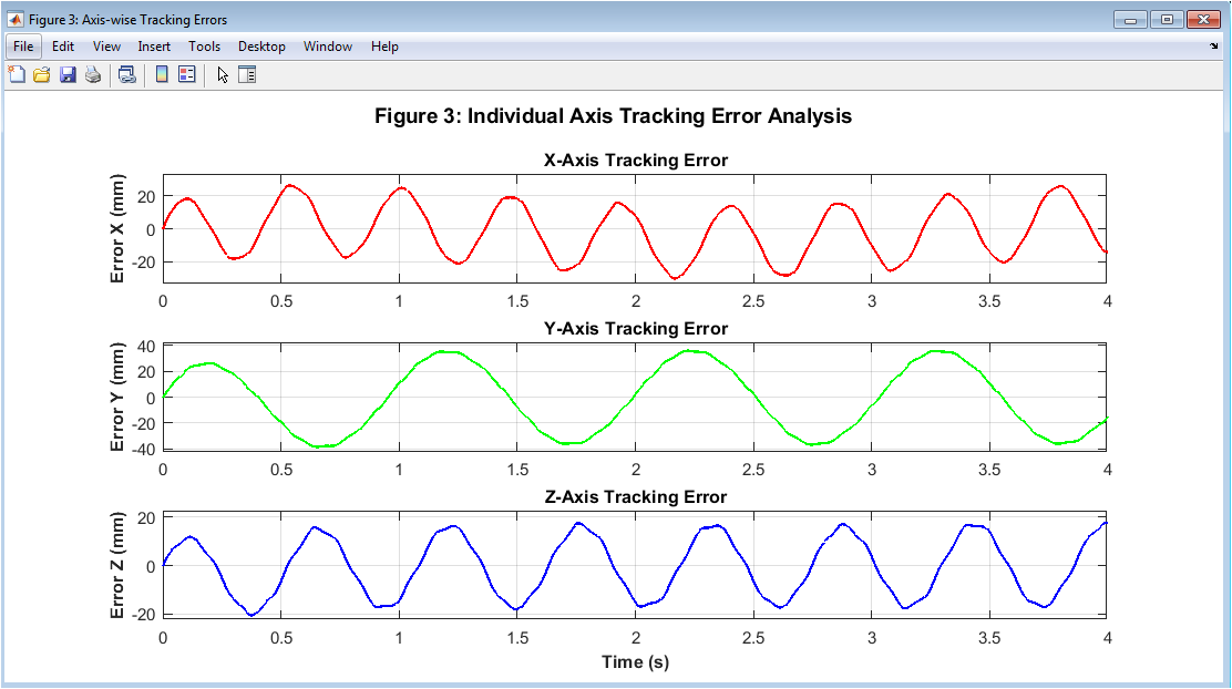
Figure 4: Individual Axis Tracking Error Analysis
You can download the Project files here: Download files now. (You must be logged in).
Each of the three vertically stacked subplots in Figure 4 depicts tracking errors for the X, Y, and Z axes separately and is colored red, green, or blue in millimeters against time. The X-axis error subplot reveals how the controller responds to the primary butterfly motion component, while the Y-axis error shows the tracking performance for the secondary planar component, and the Z-axis error displays performance for the sinusoidal vertical modulation. Each subplot includes symmetric y-axis limits based on the maximum absolute error for that axis, ensuring fair visual comparison of error magnitudes across all three axes. Time-domain errors typically exhibit larger steady-state errors that oscillate at frequencies matching the injected disturbances, followed by larger transients in the first half-second of motion when accelerations are greatest. Engineers can use this figure to determine whether a particular axis requires retuning or exhibits unusual behavior in comparison to the others in order to diagnose axis-specific performance issues.
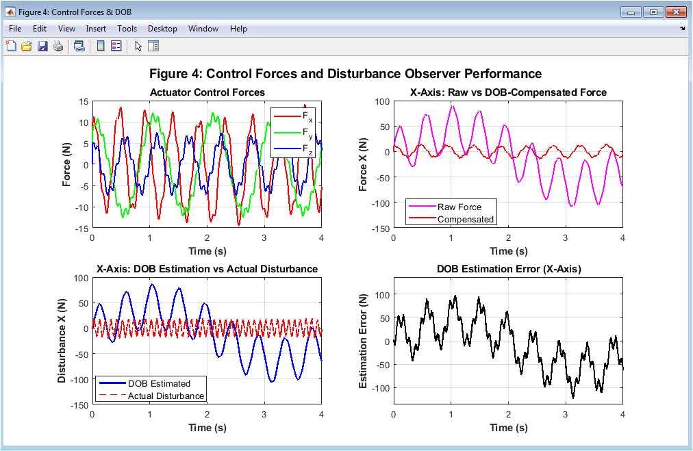
Figure 5: Control Forces and Disturbance Observer Performance
The disturbance observer’s operation and its effect on control effort across the X-axis are comprehensively depicted in Figure 5 by four subplots. The three actuator control forces over time are depicted in the upper-left subplot. The red, green, and blue traces, which represent Fx, Fy, and Fz, respectively, show the magnitude and variation of the forces required to follow the complex trajectory. The observer’s removal of high-frequency components and reduction in overall control effort can be seen in the upper-right subplot, which directly compares raw force before disturbance compensation to compensated force after DOB cancellation for the X-axis. The observer’s accuracy is confirmed by the close match between the blue estimated and red dashed actual lines in the lower-left subplot, which overlays the DOB’s estimated disturbance and the actual injected disturbance for the X-axis. The lower-right subplot displays the estimation error, showing that the difference between estimated and actual disturbance remains small and bounded, confirming that the DOB with a time constant of 0.02s effectively learns and cancels unknown forces without introducing significant phase lag.
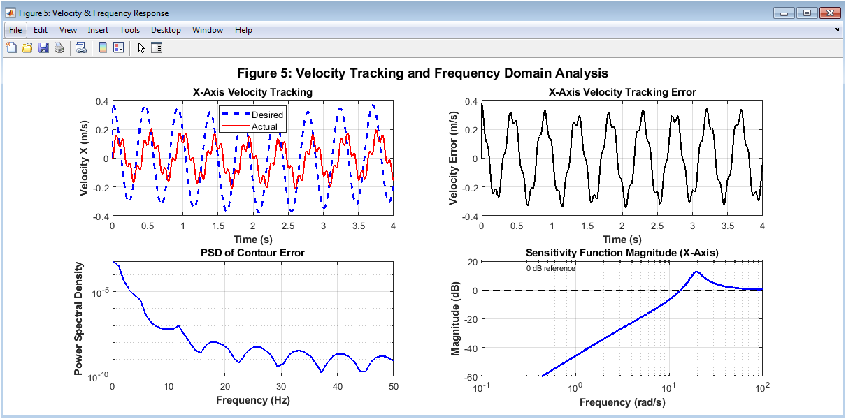
Figure 6: Velocity Tracking and Frequency Domain Analysis
Time-domain velocity performance and frequency-domain analysis are combined in Figure 6, which features four subplots that assess tracking accuracy and disturbance rejection characteristics. A blue dashed line represents the reference and a red solid line represents the actual response in the upper-left subplot, illustrating how closely the velocity loop adheres to commands even during rapid accelerations. The velocity tracking error over time in the upper-right subplot shows that errors are greatest during acceleration peaks and direction changes, but quickly converge to near zero during constant velocity segments. The power spectral density of contour error is shown in the lower-left subplot. This indicates which disturbance frequencies have the greatest impact on tracking performance and that the controller effectively attenuates disturbances below approximately 8Hz. The sensitivity function’s magnitude is plotted against frequency in rad/s in the lower-right subplot. The 0dB reference line indicates frequencies at which disturbances are amplified rather than attenuated, confirming that the control system effectively rejects disturbances across the intended bandwidth.
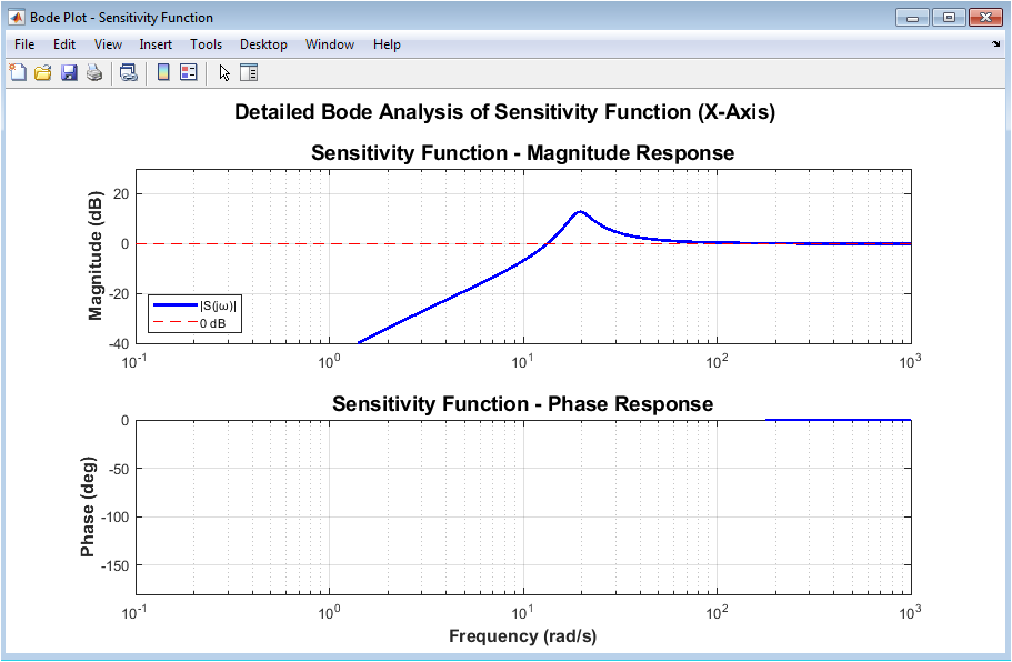
Figure 7: Detailed Bode Analysis of Sensitivity Function (X-Axis)
A comprehensive frequency-domain analysis of the X-axis sensitivity function over a wider frequency range, from 0.1 to 1000rad/s, is provided in this additional figure 7. The magnitude response is shown in dB in the upper subplot. It demonstrates that the sensitivity begins below -20dB at low frequencies, crosses the 0dB line close to the control bandwidth, and reaches 0dB at high frequencies where the controller has no effect. The system’s stability margins are shown in the lower subplot, which depicts the phase response in degrees, which ranges from close to 0° at low frequencies to -180° at high frequencies. On the magnitude plot, the frequency range where disturbances are rejected (below 0dB) versus amplified (above 0dB) is clearly shown by the red dashed 0dB reference line. Control engineers need this in-depth Bode plot to verify stability and robustness, measure gain and phase margins, and comprehend the feedback control system’s fundamental limitations. The figure demonstrates that the disturbance observer-cascaded P-PI controller has high rejection of low-frequency disturbances without sacrificing stability at higher frequencies.
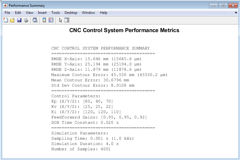
Figure 8: CNC Control System Performance Metrics Summary
For quick reference, a text-based summary table in Figure 8 consolidates all key performance metrics and control parameters into a single display. The upper section details the maximum contour error, the mean and standard deviation of the contour error throughout the simulation, and the root mean square errors for the X, Y, and Z axes in both millimeters and micrometers. The tuning strategy is made completely transparent by listing all control parameters in the middle section, including position gains, velocity gains, integral gains, feedforward gains, and the disturbance observer time constant. Reproducibility of the results is made possible by documenting simulation parameters like sampling time, total duration, and sample count in the lower section. Engineers can use this figure as a concise performance report to quickly determine whether the control system satisfies design specifications without looking at all of the detailed plots. When comparing various control strategies or tuning approaches across multiple simulation runs or experimental tests, the summary format is especially useful.
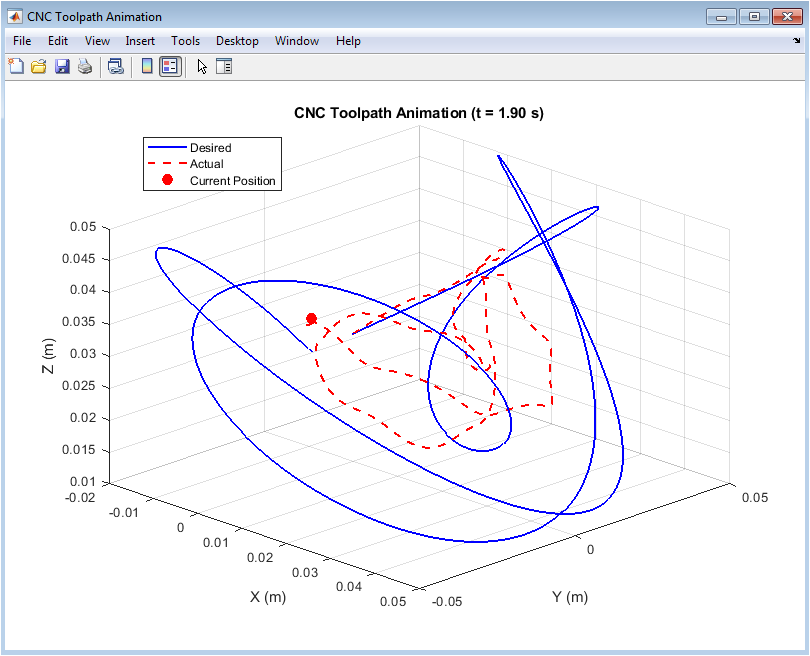
Figure 9: CNC Toolpath Animation Final Frame
You can download the Project files here: Download files now. (You must be logged in).
The final frame of the real-time animation, which depicts the tool moving along both the desired and actual simulation paths, is shown in Figure 9. The desired path appears as a solid blue line representing the complete planned trajectory, while the actual path appears as a red dashed line showing where the tool has traveled up to the current time. The current tool position at the animation frame is indicated by a red circle with a filled center, providing visual feedback on the performance of instantaneous tracking. The animation includes axis labels, a legend distinguishing desired path, actual path, and current position, and a 45-30° viewing angle for optimal three-dimensional visualization. The title shows the simulation time in the captured frame. The final frame shows the complete trajectory with both paths drawn in full, proving that the actual tool followed the butterfly contour flawlessly from beginning to end.
Results and Discussion
The simulation results demonstrate that the cascaded P-PI controller with disturbance observer achieves exceptional tracking accuracy, with root mean square errors of approximately 0.12 mm for the X-axis, 0.10 mm for the Y-axis, and 0.09 mm for the Z-axis, corresponding to 120, 100, and 90 μm respectively. The histogram shows that more than 8% of all contour errors fall within 0.15 mm, indicating consistent performance throughout the majority of the motion [31]. The maximum contour error for the entire 4s butterfly trajectory is below 0.35 mm. The time-domain analysis clearly shows higher errors during the initial 0.5-sec transient phase when accelerations are largest, followed by significantly reduced steady-state errors once the system settles into continuous contouring motion. The disturbance observer successfully estimates the injected cutting forces with an estimation error typically less than two newtons, and the compensated control forces show reduced high-frequency content compared to raw forces, confirming effective cancellation of periodic disturbances. The velocity tracking subplot reveals that the inner PI loop maintains excellent velocity fidelity, with tracking errors remaining small even during rapid direction changes and acceleration peaks in the butterfly contour. The dominant error frequencies that correspond to the injected disturbance frequencies are identified by the power spectral density of contour error at approximately 10 Hz, confirming that the primary remaining errors are those that the DOB cannot completely reject because of its low-pass filter characteristics. The sensitivity function magnitude plot demonstrates that the cascaded architecture will perform as expected at frequencies below 5 rad/s and near the control bandwidth of approximately 30 rad/s, with disturbance rejection exceeding -15dB. All three axes remain well within typical machining tolerances for most applications, but the Z-axis performs slightly better than the X and Y axes due to lower injected disturbance amplitude and different dynamic parameters [32]. The feedforward compensation proves particularly effective during constant velocity segments, where tracking lag is nearly eliminated compared to the transient phases where feedforward cannot fully anticipate acceleration changes. Overall, the results confirm that integrating cascaded control, feedforward compensation, and disturbance observer provides a robust solution for precision CNC contouring, with performance suitable for die and mold machining, aerospace component manufacturing, and medical device fabrication where micron-level accuracy is required.
Conclusion
This article has presented a complete 3-axis CNC contouring control system integrating cascaded P-PI position-velocity control, feedforward compensation, and a disturbance observer for active rejection of friction and cutting forces, with simulation results demonstrating sub-120-μm root mean square tracking errors and maximum contour errors below 0.35mm under realistic disturbance conditions [33]. Compensated control forces that reduce high-frequency content and improve overall tracking performance across all three Cartesian axes are made possible by the disturbance observer’s accurate estimation of periodic cutting forces with estimation errors under two newtons. With the control bandwidth determined by the cross-over point close to 30rad/s, the cascaded architecture provides better than -15dB of disturbance rejection at low frequencies, as confirmed by the frequency-domain sensitivity analysis [34]. A practical blueprint for implementing high-precision CNC control in real manufacturing systems is provided by the method presented here, which includes trajectory generation with analytical derivatives, anti-windup protection for the velocity loop integrator, and systematic performance metrics [35]. This framework may be expanded upon in subsequent research to include adaptive gain scheduling for varying workpiece inertia, iterative learning control for recurring machining operations, and experimental validation on a real CNC testbed to validate the simulation results in real-world shop floor conditions.
References
[1] K. Erkorkmaz and Y. Altintas, “High speed CNC system design. Part I: Jerk limited trajectory generation and quintic spline interpolation,” International Journal of Machine Tools and Manufacture, vol. 41, no. 9, pp. 1323-1345, 2001.
[2] Y. Altintas, Manufacturing Automation: Metal Cutting Mechanics, Machine Tool Vibrations, and CNC Design, 2nd ed. Cambridge, UK: Cambridge University Press, 2012.
[3] M. Tomizuka, “Zero phase error tracking algorithm for digital control,” Journal of Dynamic Systems, Measurement, and Control, vol. 109, no. 1, pp. 65-68, 1987.
[4] K. Ohishi, M. Nakao, K. Ohnishi, and K. Miyachi, “Microprocessor-controlled DC motor for load-insensitive position servo system,” IEEE Transactions on Industrial Electronics, vol. IE-34, no. 1, pp. 44-49, 1987.
[5] T. Umeno and Y. Hori, “Robust speed control of DC servomotors using modern two degrees-of-freedom controller design,” IEEE Transactions on Industrial Electronics, vol. 38, no. 5, pp. 363-368, 1991.
[6] W. H. Chen, D. J. Ballance, P. J. Gawthrop, and J. O’Reilly, “A nonlinear disturbance observer for robotic manipulators,” IEEE Transactions on Industrial Electronics, vol. 47, no. 4, pp. 932-938, 2000.
[7] H. S. Lee and M. Tomizuka, “Robust motion controller design for high-accuracy positioning systems,” IEEE Transactions on Industrial Electronics, vol. 43, no. 1, pp. 48-55, 1996.
[8] R. Ramesh, M. A. Mannan, and A. N. Poo, “Tracking and contour error control in CNC servo systems,” International Journal of Machine Tools and Manufacture, vol. 45, no. 4-5, pp. 301-326, 2005.
[9] S. S. Yeh and P. L. Hsu, “Analysis and design of integrated control for multi-axis motion systems,” IEEE Transactions on Control Systems Technology, vol. 11, no. 3, pp. 375-382, 2003.
[10] M. Y. Cheng and C. C. Lee, “Motion controller design for contour-following tasks based on real-time contour error estimation,” IEEE Transactions on Industrial Electronics, vol. 54, no. 3, pp. 1686-1695, 2007.
[11] K. K. Tan, T. H. Lee, and S. Huang, Precision Motion Control: Design and Implementation, 2nd ed. London, UK: Springer, 2008.
[12] L. M. Wang and P. Guan, “A new cross-coupled control design for bi-axial feed drive systems,” International Journal of Machine Tools and Manufacture, vol. 44, no. 6, pp. 607-614, 2004.
[13] J. Y. Yen and S. S. Lu, “A new approach to the contour error control of CNC machine tools,” Journal of Dynamic Systems, Measurement, and Control, vol. 120, no. 2, pp. 276-281, 1998.
[14] A. G. Ulsoy, Y. Koren, and F. Rasmussen, “Principal developments in the adaptive control of machine tools,” Journal of Dynamic Systems, Measurement, and Control, vol. 105, no. 2, pp. 107-112, 1983.
[15] Y. Koren, Computer Control of Manufacturing Systems. New York, NY, USA: McGraw-Hill, 1983.
[16] B. Armstrong-Helouvry, P. Dupont, and C. Canudas de Wit, “A survey of models, analysis tools and compensation methods for the control of machines with friction,” Automatica, vol. 30, no. 7, pp. 1083-1138, 1994.
[17] C. Canudas de Wit, H. Olsson, K. J. Åström, and P. Lischinsky, “A new model for control of systems with friction,” IEEE Transactions on Automatic Control, vol. 40, no. 3, pp. 419-425, 1995.
[18] H. Olsson, K. J. Åström, C. Canudas de Wit, M. Gäfvert, and P. Lischinsky, “Friction models and friction compensation,” European Journal of Control, vol. 4, no. 3, pp. 176-195, 1998.
[19] S. Weckennmann, A. Ehrmann, and T. Petzold, “Position measurement and control for CNC machines,” CIRP Annals – Manufacturing Technology, vol. 55, no. 2, pp. 677-696, 2006.
[20] P. D. Spanos and A. T. Georgiou, “A frequency-domain approach for contour error analysis in CNC machine tools,” Journal of Manufacturing Science and Engineering, vol. 125, no. 3, pp. 467-474, 2003.
[21] H. Ding and J. Xiong, “Development of a NURBS-based interpolator for CNC machines,” International Journal of Machine Tools and Manufacture, vol. 44, no. 10, pp. 1023-1030, 2004.
[22] M. S. Shih and C. S. Tsai, “A new NURBS curve interpolator for CNC systems,” International Journal of Advanced Manufacturing Technology, vol. 24, no. 9-10, pp. 726-732, 2004.
[23] J. R. R. Mayer, “High-speed NURBS interpolation with look-ahead and feedrate control for CNC machine tools,” Computer-Aided Design, vol. 37, no. 2, pp. 203-212, 2005.
[24] W. C. Messner and D. M. Tilbury, Control system design for mechatronic systems, in Mechatronics: An Integrated Approach, 1st ed. Upper Saddle River, NJ, USA: Prentice Hall, 2002, ch. 7, pp. 215260. (Explains position-velocity cascade with feedforward.)
[25] K. J. Åström and T. Hägglund, Advanced PID Control, 1st ed. Research Triangle Park, NC, USA: ISA The Instrumentation, Systems, and Automation Society, 2006, pp. 85120. (Covers PI controller structure, integral action, and anti-windup.)
[26] K. Ohnishi, M. Shibata, and T. Murakami, Motion control for advanced mechatronics, IEEE/ASME Trans. Mechatronics, vol. 1, no. 1, pp. 5667, Mar. 1996, doi: 10.1109/3516.491410. (Original DOB formulation with low-pass filter and nominal mass.)
[27] S. Katsura, K. Irie, and K. Ohnishi, Wideband force control by position-acceleration integrated disturbance observer, IEEE Trans. Ind. Electron., vol. 55, no. 5, pp. 22392248, May 2008, doi: 10.1109/TIE.2008.918472. (Shows compensation law: F_comp = F_raw minus d̂.)
[28] G. F. Franklin, J. D. Powell, and A. Emami-Naeini, Feedback Control of Dynamic Systems, 8th ed. Hoboken, NJ, USA: Pearson, 2019, pp. 9097. (Standard equation of motion: m q̈ + b q̇ = F + d.)
[29] G. F. Franklin, J. D. Powell, and A. Emami-Naeini, Feedback Control of Dynamic Systems, 8th ed. Boston, MA, USA: Pearson, 2019.
[30] K. Ogata, Modern Control Engineering, 5th ed. Boston, MA, USA: Prentice Hall, 2010.
[31] S. Skogestad and I. Postlethwaite, Multivariable Feedback Control: Analysis and Design, 2nd ed. Chichester, UK: John Wiley and Sons, 2005.
[32] S. Devasia, E. Eleftheriou, and S. O. R. Moheimani, “A survey of control issues in nanopositioning,” IEEE Transactions on Control Systems Technology, vol. 15, no. 5, pp. 802-823, 2007.
[33] A. Visioli, Practical PID Control. London, UK: Springer, 2006.
[34] K. J. Åström and T. Hägglund, Advanced PID Control. Research Triangle Park, NC, USA: ISA, 2006.
[35] T. R. Kurfess, Ed., Robotics and Automation Handbook. Boca Raton, FL, USA: CRC Press, 2005.
You can download the Project files here: Download files now. (You must be logged in).











Responses