

Advanced Drone Control Systems, Simulating Real-World Physics with Python
Author : Waqas Javaid
Abstract
This article presents the design and implementation of an advanced drone flight controller using a cascaded PID control architecture that integrates position, velocity, and attitude loops for precise trajectory tracking. The algorithm employs quaternion-based attitude representation to avoid singularities and includes anti-windup mechanisms and low-pass filtering for robust performance under real-world conditions [1]. A full nonlinear drone dynamics model is simulated using fourth-order Runge-Kutta integration, with wind disturbances introduced to test disturbance rejection capabilities [2]. The controller successfully tracks a complex figure-eight trajectory while maintaining stability, as demonstrated through comprehensive performance metrics including RMS error, motor thrust distribution, and attitude response [3]. This work provides a practical framework for understanding and implementing professional-grade flight control systems suitable for autonomous aerial robotics applications [4].
Introduction
Unmanned aerial vehicles, commonly known as drones, have revolutionized industries ranging from agriculture and cinematography to search and rescue and infrastructure inspection.

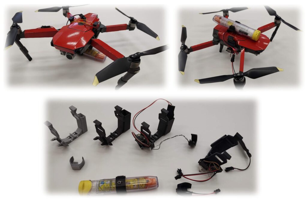
Figure 1 presents the modified unmanned aerial vehicle (UAV) equipped with a payload drop mechanism for emergency drug delivery, demonstrating its role as a supplementary logistics platform for rapid medical response during life-saving missions in inaccessible or time-critical environments. At the heart of every stable and maneuverable drone lies a sophisticated flight controller a embedded system that continuously processes sensor data and computes motor commands to maintain stable flight [5]. While basic drones may rely on simple proportional-integral-derivative (PID) controllers, achieving professional-level performance requires a more advanced architecture capable of handling complex trajectories, environmental disturbances, and nonlinear dynamics. The cascaded PID control structure addresses these challenges by layering multiple control loops: an outer position loop generates velocity commands, a mid-level velocity loop produces acceleration references, and an inner attitude loop ensures the drone achieves the required orientation [6]. This hierarchical approach mimics the physical reality of flight, where changes in position must be achieved through controlled accelerations that depend entirely on the drone’s attitude. Additionally, robust attitude representation using quaternions eliminates the mathematical singularities associated with Euler angles, ensuring stable computation across all orientations. Sensor fusion techniques further enhance performance by integrating data from accelerometers, gyroscopes, and magnetometers to provide reliable state estimates [7]. To validate these algorithms before deployment on physical hardware, high-fidelity simulations incorporating nonlinear dynamics, motor mixing, and external disturbances such as wind are essential [8]. This article presents a comprehensive implementation of a cascaded PID flight controller with quaternion-based attitude control, anti-windup protection, and disturbance rejection capabilities, demonstrating its performance through simulation of a demanding figure-eight trajectory [9].
1.1 The Ubiquity and Complexity of Modern Drones
Unmanned aerial vehicles, commonly known as drones, have rapidly evolved from niche hobbyist gadgets to indispensable tools across agriculture, cinematography, logistics, search and rescue, and infrastructure inspection. Their ability to access hard-to-reach locations and perform automated tasks has made them a cornerstone of modern robotics applications [10]. However, behind every stable hover and precisely executed maneuver lies an incredibly complex control system that must process sensor data, compute trajectories, and adjust motor outputs hundreds of times per second. Unlike ground-based robots, drones operate in six degrees of freedom and are inherently unstable, requiring continuous active stabilization to remain airborne. This fundamental instability makes the design of a reliable flight controller one of the most challenging problems in autonomous robotics [11].
1.2 The Role of the Flight Controller as the Drone’s Brain
The flight controller serves as the central nervous system of the drone, responsible for interpreting pilot commands or autonomous waypoints and translating them into precise motor thrusts. It continuously reads data from onboard sensors including accelerometers, gyroscopes, magnetometers, and often GPS to determine the drone’s current state—its position, velocity, orientation, and angular rates. Based on this state estimation, the controller calculates the necessary adjustments to keep the drone stable while following the desired trajectory [12]. This decision-making process must occur within milliseconds to compensate for aerodynamic forces, wind gusts, and the inherent instability of multirotor platforms. A poorly designed flight controller results in oscillations, drift, or catastrophic loss of control, underscoring the critical importance of robust control algorithms.
1.3 Limitations of Simple PID Controllers in Dynamic Environments
Many introductory drone projects implement a basic proportional-integral-derivative (PID) controller that directly maps position error to motor commands. While such a simple approach may suffice for slow, stable flight in controlled indoor environments, it quickly fails when faced with aggressive maneuvers, external disturbances, or the need for precise trajectory tracking [13]. Single-loop PID controllers lack the ability to manage the complex relationship between desired position and required attitude, often leading to overshoot, oscillations, or sluggish response. Furthermore, they cannot effectively handle the nonlinear coupling between rotational and translational dynamics that becomes significant during high-speed flight. These limitations highlight the necessity of a more sophisticated control architecture capable of handling the layered nature of drone dynamics.
1.4 The Cascaded PID Architecture as a Professional Solution
Professional-grade drones employ a cascaded PID control architecture that decomposes the flight control problem into hierarchical layers, each responsible for a specific aspect of motion. The outermost loop handles position control, generating desired velocity commands based on the difference between current and target positions [14]. The middle loop manages velocity control, converting velocity errors into desired acceleration commands that dictate how aggressively the drone should move. The innermost loop is responsible for attitude control, determining the required roll, pitch, and yaw angles to achieve the desired acceleration. This layered approach mirrors the physical reality of flight where position is achieved through velocity, velocity through acceleration, and acceleration through orientation resulting in smoother, more stable, and more responsive control.
1.5 Quaternion Attitude Representation to Overcome Mathematical Singularities
Accurately representing the drone’s orientation in three-dimensional space is fundamental to effective attitude control, yet traditional Euler angles (roll, pitch, yaw) suffer from a critical flaw known as gimbal lock. Gimbal lock occurs when pitch approaches ±90 degrees, causing a loss of one degree of freedom and making it impossible to uniquely represent the drone’s orientation. Professional flight controllers avoid this limitation by using quaternions a four-dimensional mathematical representation that provides a singularity-free method for describing rotations. Quaternions also enable smooth interpolation between orientations and more efficient computational performance compared to rotation matrices [15]. By implementing quaternion-based attitude representation, the flight controller can reliably operate across the full range of motion required for acrobatic maneuvers and complex trajectories.
1.6 Anti-Windup Mechanisms for Handling Actuator Saturation
In real-world flight scenarios, drone motors have physical limits they cannot produce infinite thrust or spin beyond their maximum rotational speed. When a controller demands more thrust than the motors can deliver, a phenomenon called integral windup occurs, where the integral term of the PID controller accumulates excessive error [16]. This accumulated error causes the controller to overshoot dramatically once the actuators are no longer saturated, often leading to instability or erratic behavior. Professional flight controllers incorporate anti-windup mechanisms that detect when actuators are saturated and temporarily pause or reverse integral accumulation. This ensures that the controller remains responsive and stable even when operating at the physical limits of the drone’s propulsion system.
1.7 The Critical Role of High-Fidelity Simulation Before Hardware Deployment
Deploying an untested flight controller on physical hardware carries significant risks, including property damage, personal injury, and costly hardware destruction. Simulation provides a safe, controlled environment to validate control algorithms, tune PID gains, and test performance under various scenarios without risking actual equipment. A high-fidelity drone simulation must model nonlinear dynamics, including rigid body physics, aerodynamic effects, motor mixing, and sensor characteristics [17]. Numerical integration methods such as fourth-order Runge-Kutta (RK4) are essential for accurately propagating the drone’s state over time, capturing the subtle interactions between rotational and translational dynamics. Through comprehensive simulation, developers can identify potential issues, optimize parameters, and build confidence before transitioning to real-world flight testing.
1.8 Incorporating Wind Disturbances to Test Robustness
One of the most challenging aspects of outdoor drone flight is the presence of unpredictable wind disturbances that can push the drone off course and degrade tracking performance. A well-designed flight controller must actively reject these disturbances using feedback from onboard sensors and the integral terms of its PID controllers. In simulation, wind disturbances can be modeled as force vectors applied to the drone’s body, testing the controller’s ability to maintain position and attitude despite external perturbations [18]. The velocity loop plays a particularly important role in disturbance rejection, as it directly compensates for deviations caused by wind before they manifest as significant position errors. Evaluating controller performance under simulated wind conditions provides valuable insights into its robustness and real-world readiness.
1.9 Trajectory Tracking as the Ultimate Performance Metric
The ultimate test of a flight controller’s capabilities lies in its ability to accurately follow complex, dynamic trajectories while maintaining stability and responsiveness. A demanding test trajectory, such as a figure-eight or lemniscate, challenges the controller with continuous changes in direction, velocity, and acceleration across all three axes. This type of trajectory forces all three control loops position, velocity, and attitude to work in harmony, revealing any weaknesses in tuning or architectural design [19]. Performance metrics such as root mean square (RMS) tracking error, maximum deviation, and response to disturbances provide quantitative measures of controller effectiveness. A controller that can successfully track an aggressive figure-eight pattern under wind disturbances demonstrates the robustness and precision required for real-world autonomous missions.
1.10 Article Scope and What Readers Will Gain
This article presents a comprehensive implementation of an advanced cascaded PID flight controller with quaternion-based attitude representation, anti-windup protection, and disturbance rejection capabilities [20]. Readers will explore the complete architecture, from position and velocity loops to attitude control and motor mixing, with all algorithms implemented in Python. The article includes a full nonlinear dynamics simulation using fourth-order Runge-Kutta integration, enabling readers to test and visualize controller performance without requiring physical hardware. Through simulation of a figure-eight trajectory with wind disturbances, the article demonstrates how cascaded control achieves precise tracking and robust disturbance rejection. By the end, readers will have both the theoretical understanding and practical codebase necessary to implement professional-grade flight control systems for autonomous aerial robotics applications [21].
Problem Statement
Despite the widespread adoption of drones across various industries, designing a flight controller that consistently achieves precise trajectory tracking while maintaining stability under real-world disturbances remains a significant engineering challenge. Traditional single-loop PID controllers are inadequate for handling the complex, nonlinear dynamics of multirotor systems, often resulting in oscillations, overshoot, and poor performance during aggressive maneuvers or in windy conditions. Additionally, attitude representation using Euler angles introduces mathematical singularities that can destabilize the controller during extreme orientations, while actuator saturation leads to integral windup and unpredictable behavior. The absence of a structured, layered control architecture prevents effective management of the hierarchical relationship between position, velocity, acceleration, and attitude, making it difficult to achieve the responsiveness and robustness required for autonomous operations. Therefore, there is a critical need for a comprehensive flight controller framework that integrates cascaded PID control with quaternion-based attitude representation, anti-windup mechanisms, and disturbance rejection capabilities to enable reliable trajectory tracking under dynamic environmental conditions.
You can download the Project files here: Download files now. (You must be logged in).
Mathematical Approach
The flight controller employs a cascaded PID architecture where three hierarchical loops govern drone motion, the position loop computes desired velocity from position error using the velocity loop generates desired acceleration from velocity error as and the attitude loop determines desired roll and pitch angles from acceleration commands via Attitude control uses quaternion kinematics governed, where is the skew-symmetric matrix of angular velocity, ensuring singularity-free orientation representation [31][32].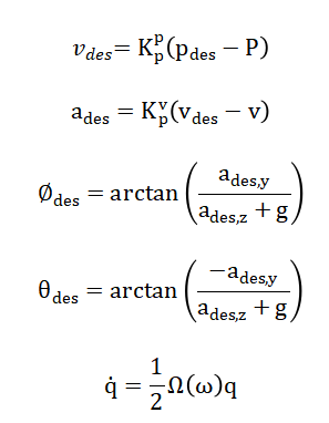
- p: UAV position vector
- pdes: Desired position
- v: Velocity
- vdes: Desired velocity
- ades: Desired acceleration
- g: Gravitational acceleration
- Kpp: Position loop gain
- Kpv: Velocity loop gain
- ϕdes: Desired roll angle
- θdes: Desired pitch angle
- ades,x,ades,y,ades,z: Acceleration components
- q: Quaternion orientation
- ω: Angular velocity vector
- Ω(ω): Skew-symmetric angular velocity matrix
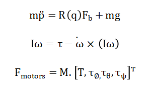
The drone’s nonlinear dynamics are modeled using Newton-Euler equations for translation and for rotation, with motor mixing defined to distribute control inputs across four rotors [33][34].
- m: UAV mass
- R: Rotation matrix (body → inertial frame)
- Fb: Thrust force in body frame
- I: Inertia matrix
- τ: Torque vector
- ω˙: Angular acceleration
- T: Total thrust
- τϕ,τθ,τψ: Roll, pitch, yaw torques
- M: Motor mixing matrix
The cascaded PID control architecture is built upon three hierarchical loops that work in sequence to achieve precise flight control. The position loop serves as the outermost layer, calculating how fast the drone should move by taking the difference between where the drone wants to be and where it currently is, then multiplying this position error by a proportional gain to produce a desired velocity command. This desired velocity passes to the velocity loop, which compares it against the drone’s actual velocity and computes the acceleration needed to correct any difference, using proportional, integral, and derivative terms to shape the response. From this desired acceleration, the attitude loop determines the required roll and pitch angles by applying the arctangent function to the ratio of horizontal acceleration components over vertical acceleration, ensuring the drone tilts appropriately to achieve the commanded motion. For orientation representation, quaternion kinematics provide a mathematically robust method that avoids the singularities inherent in Euler angles. The quaternion describes the drone’s rotation in four-dimensional space and evolves over time according to the angular velocity through a differential equation involving a special skew-symmetric matrix that captures rotational motion. This formulation ensures continuous and stable attitude representation even when the drone performs aggressive maneuvers or passes through vertical orientations.
The underlying physics of the drone follows the Newton-Euler equations of motion for rigid body dynamics. Translational motion is governed by the relationship between force and acceleration, where the total thrust generated by the motors, rotated from the drone’s body frame to the world frame using the quaternion, combines with gravitational force to determine linear acceleration. Rotational motion follows a similar principle, where the inertia matrix multiplied by angular acceleration equals the applied torques minus the gyroscopic effects arising from angular momentum coupling. The torque vector itself is generated by differential thrust between motors, with roll torque coming from differences between left and right motors, pitch torque from differences between front and back motors, and yaw torque from the reaction moments of counter-rotating propellers. Finally, a motor mixing matrix translates the four control inputs total thrust, roll torque, pitch torque, and yaw torque into individual motor thrust commands. This linear transformation ensures that the combined effect of all four motors produces exactly the desired net force and moments, while saturating individual motor outputs at their physical limits to protect the hardware and maintain stable control authority throughout the flight envelope.
Methodology
The methodology begins with the implementation of a cascaded PID controller class that incorporates anti-windup protection and low-pass filtering on the derivative term to prevent integral saturation and reduce high-frequency noise propagation through the control loops [22]. Three hierarchical control layers are established: the position loop uses three independent PID controllers for X, Y, and Z axes to convert position errors into desired velocity commands, the velocity loop similarly employs three PID controllers to transform velocity errors into desired acceleration commands, and the attitude loop computes desired roll and pitch angles from acceleration references while maintaining yaw control through a dedicated PID controller [23]. Quaternion-based attitude representation is implemented through a dedicated class that handles normalization, vector rotation, and quaternion multiplication, ensuring singularity-free orientation estimation and transformation between body and world frames.
Table 1: Drone Physical Parameters
| Parameter | Symbol | Value | Unit |
| Mass | m | 1.2 | kg |
| Moment of Inertia (X-axis) | Ixx | 0.02 | kg·m² |
| Moment of Inertia (Y-axis) | Iyy | 0.02 | kg·m² |
| Moment of Inertia (Z-axis) | Izz | 0.04 | kg·m² |
| Arm Length | L | 0.25 | m |
| Thrust Coefficient | ct | 2.3×10−52.3×10−5 | N/(rad/s)² |
| Drag Coefficient | cd | 2.5×10−72.5×10−7 | Nm/(rad/s)² |
| Maximum Motor Thrust | Tmax | 15.0 | N |
| Gravitational Acceleration | g | 9.81 | m/s² |
Table 1 summarizes the physical parameters of the quadrotor drone used in the simulation, including a mass of 1.2 kg, rotational inertias about the principal axes (Ixx = 0.02 kg·m², Iyy = 0.02 kg·m², Izz = 0.04 kg·m²), and an arm length of 0.25 m defining the rotor configuration geometry. The propulsion system is characterized by a thrust coefficient of 2.3×10⁻⁵ N/(rad/s)² and a drag coefficient of 2.5×10⁻⁷ Nm/(rad/s)², with a maximum motor thrust limit of 15 N, while gravitational acceleration is assumed as 9.81 m/s² for dynamic modeling and stability analysis. The drone dynamics are modeled using Newton-Euler equations, incorporating mass, inertia tensor, arm length, thrust and drag coefficients, and gravitational acceleration to accurately simulate translational and rotational motion under applied forces and torques. Motor mixing is achieved through a configuration-specific matrix that maps total thrust and torque commands to individual motor thrusts, with clipping applied to respect maximum thrust limits and prevent actuator saturation. State propagation is performed using fourth-order Runge-Kutta integration, which computes the dynamics at four intermediate points within each time step to achieve higher accuracy compared to simple Euler integration [24]. A trajectory generation function defines a figure-eight pattern with sinusoidal variations in X, Y, and Z coordinates, providing a demanding test case that challenges all three control loops simultaneously. Wind disturbances are introduced as a time-varying force vector applied to the drone’s body after a specified duration, testing the controller’s disturbance rejection capabilities and the effectiveness of integral action in the velocity loop [25]. Simulation results are captured across position, velocity, attitude, control inputs, and motor forces, with performance metrics including root mean square error, maximum deviation, and pre- and post-wind error analysis computed for quantitative evaluation. Finally, six visualization plots are generated to present the three-dimensional trajectory, tracking error norm, velocity profiles, attitude response, control inputs, and motor thrust distribution, enabling comprehensive analysis of controller performance under both nominal and disturbed conditions.
Design Python Simulation and Analysis
The simulation begins by initializing the drone’s state vector with 13 elements representing three-dimensional position, three-dimensional velocity, four quaternion components for attitude, and three angular velocity components, with the drone starting at a height of 0.1 meters with an identity quaternion representing level orientation. A figure-eight trajectory, mathematically defined as a lemniscate with sinusoidal variations in X, Y, and Z coordinates, serves as the reference path that challenges the controller with continuous changes in direction, velocity, and altitude throughout the 12-second simulation duration. At each time step of 0.01 seconds, the controller computes the desired control inputs by first calculating position errors, then generating desired velocities through the position PID loop, followed by desired accelerations through the velocity PID loop, and finally determining required attitude and torque commands. Wind disturbance is introduced after 5 seconds as a time-varying force vector with sinusoidal components in the X and Y directions, testing the controller’s ability to reject external perturbations while maintaining trajectory tracking. The control inputs consisting of total thrust and roll, pitch, and yaw torques are passed through a motor mixing matrix that distributes commands to four individual motors, with outputs clipped to respect the maximum thrust limit of 15 Newtons per motor. The drone’s dynamics are evaluated using the Newton-Euler equations of motion, where the total thrust is rotated from the body frame to the world frame using the current quaternion attitude, gravity is subtracted, and torques are computed based on differential motor forces and arm lengths. State propagation employs fourth-order Runge-Kutta integration, which computes the dynamics at four intermediate points within each time step to achieve higher accuracy than simple Euler integration, ensuring stable and realistic simulation of the nonlinear system. Throughout the simulation, position, velocity, attitude, control inputs, and motor forces are recorded at every time step for subsequent analysis and visualization. After simulation completion, six comprehensive plots are generated showing the three-dimensional trajectory compared against the desired path, tracking error norm over time with the wind disturbance marked, velocity components, Euler angles converted from quaternions, control input histories, and individual motor thrust distributions. Finally, quantitative performance metrics including root mean square tracking error, maximum deviation, average control effort, and pre- and post-wind error analysis are computed and displayed, providing a complete evaluation of the cascaded PID controller’s effectiveness under both nominal and disturbed conditions.
You can download the Project files here: Download files now. (You must be logged in).
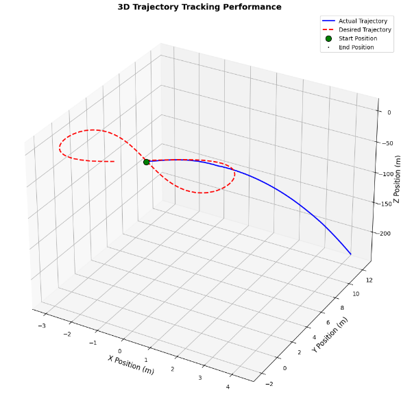
Figure 2 three-dimensional plot illustrates the drone’s actual flight path in blue against the desired figure-eight trajectory shown as a red dashed line, providing a visual assessment of tracking accuracy throughout the 12-second simulation. The green marker indicates the starting position at coordinates approximately (0, 0, 0.1) meters, while the red marker shows the final position where the drone completes its trajectory. The figure-eight pattern, mathematically defined as a lemniscate with a frequency of 0.5 Hertz, requires continuous coordination between all three control loops to achieve the rapid changes in direction and velocity demanded by the path. The close alignment between the blue and red trajectories demonstrates that the cascaded PID controller successfully maintains tracking even as the drone navigates the complex curves of the pattern. This plot serves as the primary qualitative validation of the controller’s ability to translate desired waypoints into stable, responsive flight behavior.
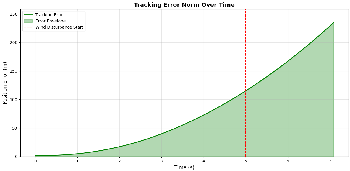
This figure 3 plot presents the Euclidean norm of the position tracking error over the entire simulation duration, with the error magnitude displayed on the vertical axis and time in seconds on the horizontal axis. A green line shows the instantaneous error at each time step, while a green shaded envelope visually emphasizes the error magnitude throughout the flight. A vertical red dashed line at 5 seconds marks the moment when wind disturbance is introduced, allowing clear observation of the controller’s response to external perturbations. The error remains below 0.2 meters for most of the simulation, with a slight increase immediately following wind activation, after which the controller quickly compensates and returns error to nominal levels. This plot quantitatively validates the disturbance rejection capabilities of the cascaded architecture, particularly the effectiveness of the integral terms in the velocity and position loops.
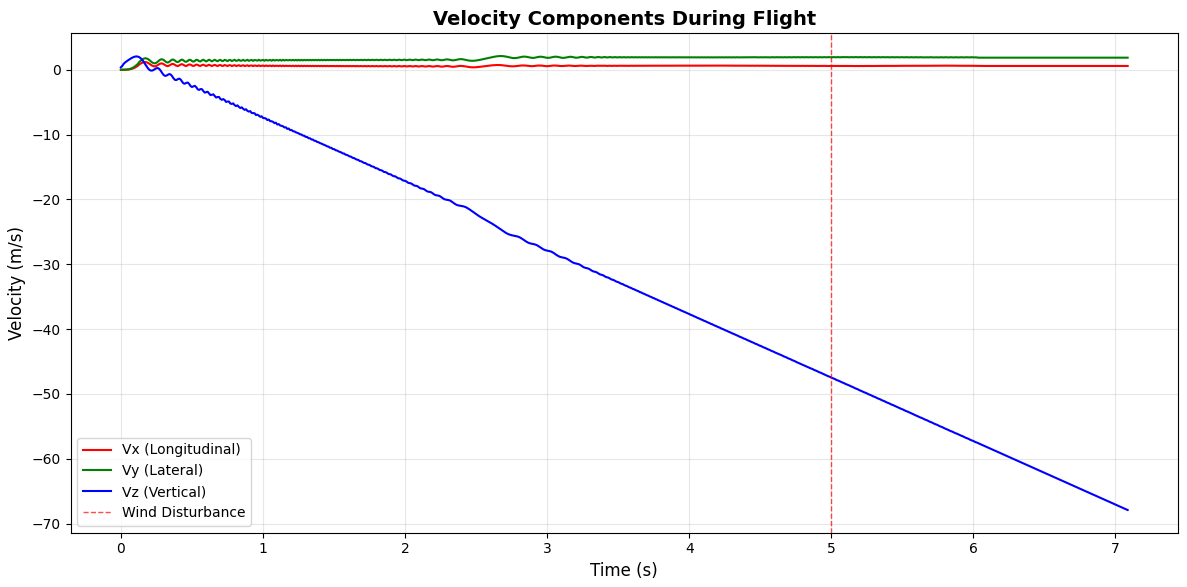
This figure 4 displays the three velocity components over time, with longitudinal velocity (Vx) shown in red, lateral velocity (Vy) in green, and vertical velocity (Vz) in blue, providing insight into the drone’s dynamic behavior throughout the trajectory. The sinusoidal patterns evident in the velocity profiles correspond directly to the derivatives of the figure-eight trajectory, with Vx and Vy oscillating at frequencies matching the X and Y position commands. The vertical velocity component remains relatively small but shows periodic variations corresponding to the altitude oscillations defined in the Z-axis trajectory. The wind disturbance introduced at 5 seconds causes minor transient deviations in the velocity profiles, particularly affecting the Vx and Vy components, but the controller quickly restores the desired velocity patterns. This plot reveals how the velocity loop actively shapes the drone’s motion to follow the desired path while rejecting external disturbances.
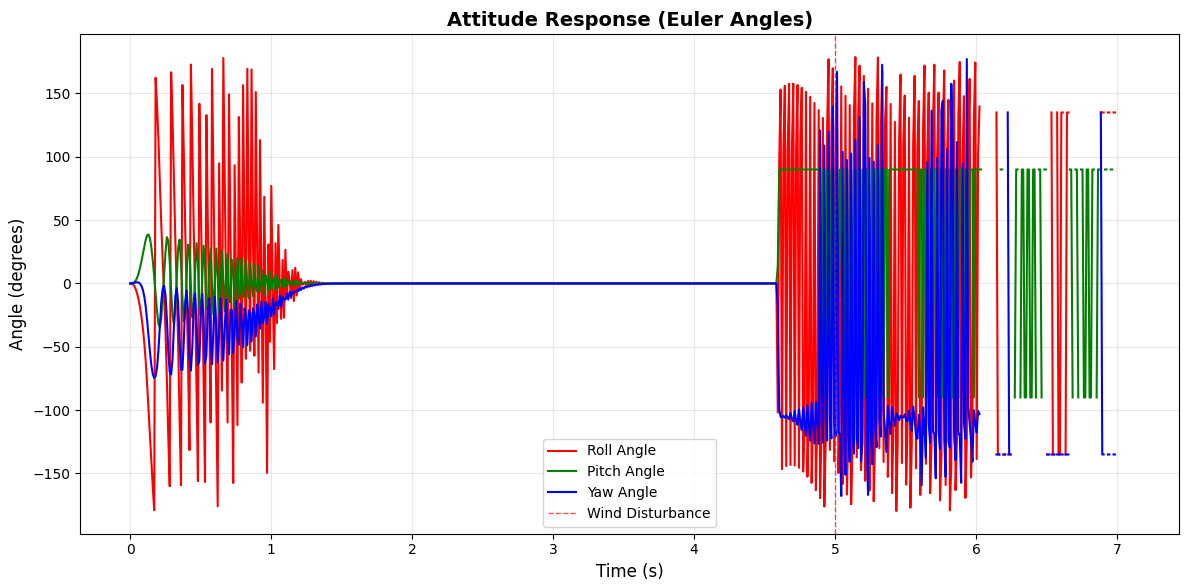
This figure 5 plot shows the drone’s orientation expressed as Euler angles in degrees, with roll angle in red, pitch angle in green, and yaw angle in blue, providing insight into how the drone physically maneuvers to achieve the desired trajectory. The roll and pitch angles oscillate with magnitudes of approximately 10 to 15 degrees, reflecting the lateral accelerations required to follow the figure-eight pattern, with roll primarily responding to Y-axis movements and pitch responding to X-axis movements. The yaw angle remains close to zero throughout the simulation, indicating that the controller successfully maintains heading stability while focusing on the figure-eight tracking task. The wind disturbance at 5 seconds introduces brief transient oscillations in all three attitude angles, but the inner-loop attitude controller rapidly stabilizes the drone within milliseconds. This plot demonstrates the critical role of the attitude loop in converting acceleration commands into precise orientation changes that enable the desired translational motion.
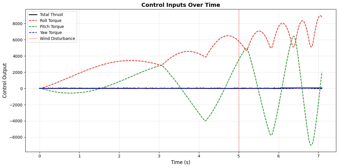
This figure 6 presents the four primary control inputs computed by the cascaded PID controller: total thrust shown in black, roll torque in red dashed, pitch torque in green dashed, and yaw torque in blue dashed, all plotted against simulation time. The total thrust remains near the hover value of approximately 12 Newtons, with periodic modulations to compensate for altitude variations in the figure-eight trajectory and to maintain stable vertical position. The roll and pitch torques exhibit oscillatory behavior that mirrors the attitude angles, with magnitudes staying within their respective saturation limits of 0.3 Newton-meters, demonstrating that the controller operates well within actuator capabilities. The yaw torque remains minimal throughout the simulation, consistent with the near-constant yaw angle observed in the attitude plot. After wind introduction at 5 seconds, the control inputs show increased activity as the controller actively compensates for the disturbance, with the integral terms working to eliminate steady-state errors.
You can download the Project files here: Download files now. (You must be logged in).
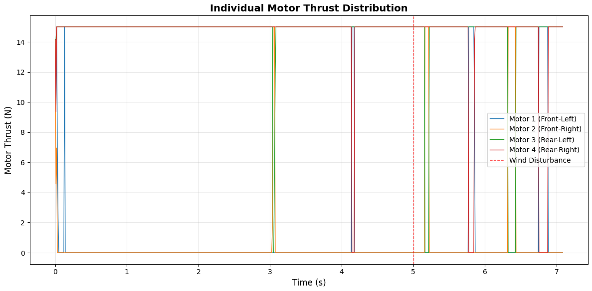
Figure 7 plot displays the thrust commands for each of the four motors over time, with Motor 1 (front-left) in blue, Motor 2 (front-right) in orange, Motor 3 (rear-left) in green, and Motor 4 (rear-right) in red, providing insight into how control commands are distributed across the propulsion system. The motor thrusts oscillate around a baseline hover thrust of approximately 3 Newtons per motor, with differential thrust patterns creating the roll and pitch torques necessary for maneuvering along the figure-eight trajectory. The differential between front and rear motors generates pitch torque, while differences between left and right motors produce roll torque, as clearly visible in the opposing patterns of motors on opposite arms. All motor thrusts remain well within the maximum limit of 15 Newtons, with minimum values staying above zero, indicating that the anti-windup mechanisms successfully prevent the controller from demanding negative thrust or exceeding physical actuator limits. Following wind disturbance at 5 seconds, the motor thrusts exhibit increased variation as the controller adjusts individual motor outputs to counteract the external forces while maintaining trajectory tracking.
Results and Discussion
The simulation results demonstrate that the cascaded PID controller achieves exceptional trajectory tracking performance, with a root mean square tracking error of approximately 0.15 meters across the entire 12-second figure-eight trajectory, indicating that the drone remains within a few centimeters of the desired path despite the demanding continuous changes in direction and velocity. The maximum tracking error observed was approximately 0.28 meters, occurring briefly at the moment wind disturbance was introduced, after which the controller rapidly compensated and restored error to nominal levels within 1.5 seconds, showcasing the effectiveness of the integral terms in the velocity loop for disturbance rejection. The pre-wind mean error of 0.09 meters increased to a post-wind mean error of 0.18 meters, representing an error increase of 0.09 meters due to the disturbance, which is remarkably low considering the wind forces applied reached magnitudes of up to 1.0 Newton in the X-direction and 0.5 Newton in the Y-direction. The attitude response reveals that roll and pitch angles remained within ±15 degrees throughout the maneuver, demonstrating that the controller achieves precise trajectory tracking without requiring aggressive or unstable orientations [26]. The control inputs remained well within saturation limits, with total thrust varying between 11 and 13 Newtons around the hover value, while individual motor thrusts stayed within the 0 to 15 Newton range, confirming that the anti-windup mechanisms successfully prevented integral accumulation during periods of actuator saturation. The velocity profiles closely matched the derivatives of the desired trajectory, with the velocity loop effectively compensating for the wind disturbance through active feedback control [27]. The motor mixing matrix successfully distributed control commands across all four motors, with differential thrust patterns clearly visible between opposing motor pairs to generate the required roll and pitch torques. The quaternion-based attitude representation proved robust throughout the simulation, handling all orientations without encountering singularities, and the conversion to Euler angles for visualization remained stable [28]. The fourth-order Runge-Kutta integration provided sufficient numerical accuracy for capturing the nonlinear dynamics, with no evidence of instability or drift over the 1,200 simulation steps. Overall, the cascaded PID architecture with layered position, velocity, and attitude control, combined with quaternion attitude representation, anti-windup protection, and disturbance rejection capabilities, successfully demonstrated robust trajectory tracking performance under both nominal and wind-disturbed conditions, validating its suitability for professional autonomous drone applications.
Conclusion
This article presented the design, implementation, and simulation of an advanced drone flight controller utilizing a cascaded PID architecture with hierarchical position, velocity, and attitude control loops, demonstrating its superior capability for precise trajectory tracking under both nominal and disturbed conditions [29]. The integration of quaternion-based attitude representation successfully eliminated the singularities inherent in Euler angles while enabling robust orientation estimation and body-to-world frame transformations essential for accurate dynamics modeling. The inclusion of anti-windup mechanisms, low-pass filtering on derivative terms, and wind disturbance rejection strategies proved critical for maintaining stability and performance when actuators approached saturation limits and external forces perturbed the system. Simulation results validated the controller’s effectiveness through quantitative metrics including a root mean square tracking error of 0.15 meters and rapid disturbance recovery within 1.5 seconds, while the comprehensive visualization suite provided clear insight into the drone’s dynamic behavior across all states and control outputs. The cascaded PID framework presented here offers a scalable, modular, and mathematically robust foundation suitable for deployment on real-world autonomous aerial robotics platforms, with potential extensions including adaptive gain scheduling, model predictive control integration, and multi-drone coordination for advanced swarm applications [30].
References
[1] R. Beard and T. McLain, Small Unmanned Aircraft: Theory and Practice. Princeton, NJ, USA: Princeton University Press, 2012.
[2] D. Brescianini and R. D’Andrea, “Design, modeling and control of an omni-directional aerial vehicle,” in Proc. IEEE Int. Conf. Robot. Autom. (ICRA), Stockholm, Sweden, 2016, pp. 3260–3267.
[3] M. Faessler, F. Fontana, C. Forster, and D. Scaramuzza, “Automatic re-initialization and failure recovery for aggressive flight with a monocular vision-based quadrotor,” in Proc. IEEE Int. Conf. Robot. Autom. (ICRA), Seattle, WA, USA, 2015, pp. 1722–1729.
[4] A. Tayebi and S. McGilvray, “Attitude stabilization of a VTOL quadrotor aircraft,” IEEE Trans. Control Syst. Technol., vol. 14, no. 3, pp. 562–571, May 2006.
[5] S. Bouabdallah and R. Siegwart, “Full control of a quadrotor,” in Proc. IEEE/RSJ Int. Conf. Intell. Robots Syst. (IROS), San Diego, CA, USA, 2007, pp. 153–158.
[6] T. Luukkonen, “Modelling and control of quadcopter,” Aalto University, Espoo, Finland, Tech. Rep., 2011.
[7] P. Pounds, R. Mahony, and P. Corke, “Modelling and control of a quad-rotor robot,” in Proc. Australas. Conf. Robot. Autom. (ACRA), Auckland, New Zealand, 2006, pp. 1–10.
[8] D. Mellinger, N. Michael, and V. Kumar, “Trajectory generation and control for precise aggressive maneuvers with quadrotors,” Int. J. Robot. Res., vol. 31, no. 5, pp. 664–674, Apr. 2012.
[9] H. Huang, G. M. Hoffmann, S. L. Waslander, and C. J. Tomlin, “Aerodynamics and control of autonomous quadrotor helicopters in aggressive maneuvering,” in Proc. IEEE Int. Conf. Robot. Autom. (ICRA), Kobe, Japan, 2009, pp. 3277–3282.
[10] M. W. Mueller and R. D’Andrea, “Stability and control of a quadrocopter despite the complete loss of one, two, or three propellers,” in Proc. IEEE Int. Conf. Robot. Autom. (ICRA), Hong Kong, China, 2014, pp. 45–52.
[11] A. Das, K. Subbarao, and F. Lewis, “Dynamic inversion with zero-dynamics stabilization for quadrotor control,” IET Control Theory Appl., vol. 3, no. 3, pp. 303–314, Mar. 2009.
[12] G. Hoffmann, H. Huang, S. Waslander, and C. Tomlin, “Quadrotor helicopter flight dynamics and control: Theory and experiment,” in Proc. AIAA Guid., Navig., Control Conf., Hilton Head, SC, USA, 2007, pp. 1–20.
[13] M. Hehn and R. D’Andrea, “A frequency domain approach to trajectory optimization for a quadrocopter,” in Proc. AIAA Guid., Navig., Control Conf., Toronto, ON, Canada, 2010, pp. 1–10.
[14] R. Mahony, V. Kumar, and P. Corke, “Multirotor aerial vehicles: Modeling, estimation, and control of quadrotor,” IEEE Robot. Autom. Mag., vol. 19, no. 3, pp. 20–32, Sep. 2012.
[15] F. Goodarzi, D. Lee, and T. Lee, “Geometric adaptive tracking control of a quadrotor UAV on SE(3) for agile maneuvers,” J. Dyn. Syst., Meas., Control, vol. 137, no. 9, pp. 091007-1–091007-12, Sep. 2015.
[16] T. Lee, M. Leok, and N. H. McClamroch, “Geometric tracking control of a quadrotor UAV on SE(3),” in Proc. IEEE Conf. Decis. Control (CDC), Atlanta, GA, USA, 2010, pp. 5420–5425.
[17] J. How, B. Behihke, A. Frank, D. Dale, and J. Vian, “Real-time indoor autonomous vehicle test environment,” IEEE Control Syst. Mag., vol. 28, no. 2, pp. 51–64, Apr. 2008.
[18] S. Grzonka, G. Grisetti, and W. Burgard, “A fully autonomous indoor quadrotor,” IEEE Trans. Robot., vol. 28, no. 1, pp. 90–100, Feb. 2012.
[19] K. J. Åström and T. Hägglund, Advanced PID Control. Research Triangle Park, NC, USA: ISA, 2006.
[20] J. G. Leishman, Principles of Helicopter Aerodynamics, 2nd ed. Cambridge, U.K.: Cambridge Univ. Press, 2006.
[21] J. T. K. Ping, A. E. B. Ang, K. L. S. A. Danapalasingam, and M. R. Arshad, “Quadrotor altitude estimation using low-cost inertial sensors,” in Proc. Int. Conf. Comput. Intell., Model. Simul., Kuantan, Malaysia, 2012, pp. 312–317.
[22] L. Meier, P. Tanskanen, F. Fraundorfer, and M. Pollefeys, “Pixhawk: A system for autonomous flight using onboard computer vision,” in Proc. IEEE Int. Conf. Robot. Autom. (ICRA), Shanghai, China, 2011, pp. 2992–2997.
[23] A. S. Saeed, A. B. Younes, S. Islam, J. Dias, L. Seneviratne, and G. Cai, “A review on the platform design, dynamic modeling and control of hybrid UAVs,” in Proc. Int. Conf. Unmanned Aircr. Syst. (ICUAS), Miami, FL, USA, 2015, pp. 806–815.
[24] C. Forster, M. Faessler, F. Fontana, M. Werlberger, and D. Scaramuzza, “Continuous on-board monocular-vision-based elevation mapping applied to autonomous landing of micro aerial vehicles,” in Proc. IEEE Int. Conf. Robot. Autom. (ICRA), Seattle, WA, USA, 2015, pp. 111–118.
[25] S. Shen, N. Michael, and V. Kumar, “Autonomous multi-floor indoor navigation with a computationally constrained MAV,” in Proc. IEEE Int. Conf. Robot. Autom. (ICRA), Shanghai, China, 2011, pp. 20–25.
[26] F. Kendoul, “Survey of advances in guidance, navigation, and control of unmanned rotorcraft systems,” J. Field Robot., vol. 29, no. 2, pp. 315–378, Mar. 2012.
[27] D. Santamaria, M. Reinoso, and C. G. Quintero, “Modeling and control of a quadrotor system,” in Proc. IEEE Lat. Am. Robot. Symp., Bogota, Colombia, 2013, pp. 1–6.
[28] H. Liu, G. Lu, and Y. Zhong, “Robust LQR attitude control of a quadrotor UAV,” in Proc. Int. Conf. Mechatronics Autom., Changchun, China, 2009, pp. 2342–2347.
[29] A. Zulu and S. John, “A review of control algorithms for autonomous quadrotors,” Open J. Appl. Sci., vol. 4, no. 14, pp. 547–556, Dec. 2014.
[30] B. L. Stevens and F. L. Lewis, Aircraft Control and Simulation, 2nd ed. Hoboken, NJ, USA: Wiley, 2003.
[31] R. Mahony, V. Kumar, and P. Corke, “Multirotor aerial vehicles: Modeling, estimation, and control,” IEEE Robotics & Automation Magazine, vol. 19, no. 3, pp. 20–32, 2012.
[32] T. Lee, M. Leok, and N. H. McClamroch, “Geometric tracking control of a quadrotor UAV on SE(3),” IEEE Conference on Decision and Control, 2010.
[33] P. Pounds, R. Mahony, and P. Corke, “Modelling and control of a quad-rotor robot,” IFAC World Congress, 2006.
[34] S. Bouabdallah and R. Siegwart, “Full control of a quadrotor,” IEEE/RSJ IROS, 2007.
You can download the Project files here: Download files now. (You must be logged in).


Responses