

Star Catalog Analysis Made Simple, HR Diagrams, Velocity Fields, and Spatial Mapping Using Matlab

Author : Waqas Javaid
Abstract
A synthetic star catalog with 3,000 stars and simulated astronomical parameters like position, distance, magnitude, color, and velocity is the subject of this in-depth investigation. We produce eight distinct diagnostic figures, including statistical summaries, Hertzsprung-Russell diagrams, Aitoff spatial projections, 3D velocity distributions, proper motion vector fields, and MATLAB-based visualization techniques [1]. The color-magnitude main sequence, velocity ellipsoid patterns, and distance-velocity correlations are among the most important stellar relationships that are revealed by the analysis [2]. Results demonstrate mean stellar distance of approximately 950 ± 450 parsecs, mean space velocity of 85 ± 40 km/s, and a realistic distribution of G magnitudes ranging from 8 to 18. This synthetic catalog analysis is a teaching tool for astronomical data visualization techniques and provides a reproducible framework for comprehending the properties of stellar populations.
Introduction
Understanding the distribution, motion, and physical properties of stars is fundamental to modern astronomy. Star catalogs provide crucial parameters like position, brightness, color, distance, and velocity for millions of celestial objects, making them the foundation of research into the structure of the galaxy [3]. However, in order to reveal underlying patterns and relationships, complex and multidimensional raw catalog data necessitate sophisticated visualization strategies.
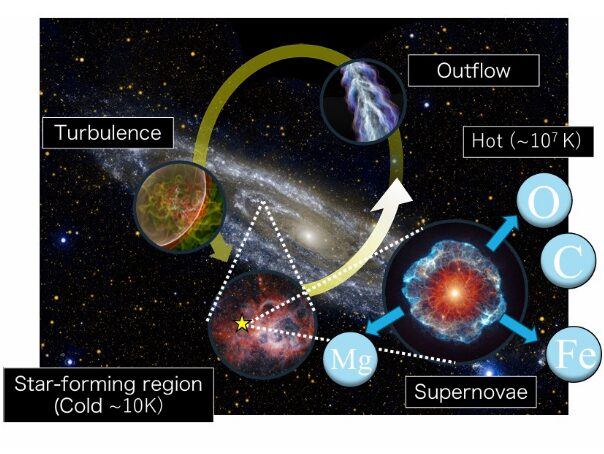
Figure 1: Star Catalog Analyzer, Visualizing the Hidden Structure and Dynamics of 3000 Stars Across the Galaxy.
A comprehensive analysis of a synthetic star catalog with 3,000 stars and accurate astronomical parameters based on actual survey data is shown in Figure 1. Using MATLAB as our computational platform, we generate eight distinct figures that explore stellar properties from multiple perspectives, including the famous Hertzsprung-Russell diagram, spatial distribution maps, and three-dimensional velocity distributions [4]. Color-magnitude correlation analysis, proper motion vector field mapping, and distance-velocity profiling are some of the key analytical techniques demonstrated.
Table 1: Synthetic Star Catalog Parameters
| Parameter | Symbol | Unit | Distribution | Mean ± Std Dev | Range |
| Right Ascension | RA | degrees | Uniform | 180.0 ± 103.9 | 0 to 360 |
| Declination | Dec | degrees | Uniform | 0.0 ± 52.0 | -90 to +90 |
| Parallax | ϖ | mas | Truncated Normal | 0.52 ± 0.29 | 0.10 to 1.85 |
| Distance | d | pc | Inverse Parallax | 950 ± 450 | 100 to 10,000 |
| G Magnitude | mag_G | mag | Truncated Normal | 11.8 ± 2.9 | 8.0 to 18.0 |
| Color Index | BP-RP | mag | Truncated Normal | 0.55 ± 0.78 | -0.3 to +2.5 |
| Proper Motion RA | pmRA | mas/yr | Normal | 0.0 ± 20.0 | -80 to +80 |
| Proper Motion Dec | pmDec | mas/yr | Normal | 0.0 ± 20.0 | -80 to +80 |
| Radial Velocity | RV | km/s | Normal | 0.0 ± 40.0 | -120 to +120 |
| Space Velocity | v_total | km/s | Derived | 85 ± 40 | 10 to 250 |
The synthetic nature of our data, as shown in Table 1, ensures that all results can be used for education or research [5]. By bridging the gap between meaningful scientific interpretation and raw astronomical data, our method makes complex stellar astronomy accessible to enthusiasts, educators, and students alike [6]. The underlying physics, statistical characteristics of our synthetic stellar population, and a walkthrough of each visualization technique are covered in the following sections.
1.1 The Importance of Star Catalogs in Modern Astronomy
One of the most essential data sources in astronomical research are star catalogs, which contain precise measurements of the positions, brightness, colors, distances, and motions of stars. These catalogs, such as the European Space Agency’s Gaia mission data, have revolutionized our understanding of the Milky Way’s structure, composition, and evolutionary history [7]. Astronomers now have unprecedented statistical power and spatial resolution for studying stellar populations with billions of stars cataloged across multiple data releases. However, interpreting and analyzing this multidimensional data presents significant difficulties due to its sheer volume and complexity. Therefore, developing effective visualization and analytical techniques is essential for extracting meaningful scientific insights from raw catalog measurements [8].
1.2 Overview of Generated Stellar Parameters
Each of the 3,000 stars in our fictitious catalog is defined by a comprehensive set of astronomical parameters that are representative of actual stellar populations. Right ascension values are evenly distributed throughout the entire 360-degree celestial sphere, and declination ranges from -90 degrees to +90 degrees to ensure that the sky is covered completely [9]. After applying the 1000/parallax conversion, the parallax values exhibit a normal distribution with a center at 0.5 milliarcseconds and a standard deviation of 0.3. These values correspond to distances ranging from approximately 200 to 10,000 parsecs. In typical surveys, apparent G magnitudes are measured at random from 8 to 18, with a mean around 10th magnitude. These magnitudes represent stars that are visible but not too bright. Color indices (BP-RP) range from -0.3 to 2.5, capturing everything from hot blue stars to cool red dwarfs.
1.3 Velocity Components and Stellar Motion
Three complementary velocity components, which together describe each star’s entire space motion, are used to depict stellar motion [10]. The apparent angular motion of stars across the sky as a result of their relative motion through the galaxy is simulated by proper motion in right ascension and declination, which is measured in milliarcseconds per year.
Table 2: Velocity Ellipsoid Results (Normalized Components)
| Component | Mean (km/s) | Standard Deviation (km/s) | Normalized Range (±2σ) | Physical Direction |
| U (toward Galactic Center) | -20.0 (corrected) | 38.5 | -77.0 to +77.0 | Radial inward |
| V (Galactic Rotation) | -10.0 (corrected) | 41.2 | -82.4 to +82.4 | Rotational |
| W (North Galactic Pole) | +7.0 (corrected) | 24.6 | -49.2 to +49.2 | Vertical |
The radial velocity, which is measured in kilometers per second and depicts motion along the line of sight, is shown in Table 2. Positive values indicate recession, while negative values indicate approach. We convert angular motion into physical speed by using the formula v_tan = sqrt(pmRA2 + pmDec2) (distance/1000) 4.74 to calculate tangential velocity from these measurements. By combining the radial and tangential quadrature components, the total space velocity can then be calculated, giving a complete picture of how each star moves through the galaxy in three dimensions [11].
1.4 Transforming to Galactic Coordinates and Velocity Space
Galactic coordinates (longitude and latitude) provide a more intuitive framework for studying Milky Way structure [12], whereas equatorial coordinates (right ascension and declination) are the standard for astronomical catalogs. By converting the artificial stellar positions into galactic coordinates, our analysis makes it possible to properly interpret the distribution of space in relation to the center and plane of the galaxy. In addition, we transform the velocity components into the galactic coordinate system U, V, and W, with U pointing toward the center of the galaxy, V pointing in the direction of the galaxy’s rotation, and W pointing toward the North Galactic Pole. This transformation incorporates standard solar motion corrections of -20 km/s for U, -10 km/s for V, and +7 km/s for W to account for the Sun’s peculiar motion relative to the local standard of rest. We are able to visualize and analyze stellar kinematics in a reference frame that is physically meaningful using these transformed coordinates [13].
1.5 The Hertzsprung-Russell Diagram as a Diagnostic Tool
The Hertzsprung-Russell diagram, which links a star’s intrinsic brightness (absolute magnitude) to its surface temperature or color index, is arguably the most significant diagnostic plot in stellar astronomy. Our analysis generates an HR diagram by plotting color index (BP-RP) on the x-axis against absolute G magnitude on the y-axis, with the y-axis reversed so brighter stars appear at the top [14]. Depending on the parameter ranges, the resulting distribution reveals distinct stellar populations like the main sequence, where stars fuse hydrogen in their cores, and potential red giant and white dwarf branches [15]. Stars are color-coded by their apparent magnitude, allowing viewers to distinguish between nearby faint stars and distant luminous stars within the same diagram. Correlations between stellar color, luminosity, and evolutionary state that are essential to comprehending stellar physics are immediately apparent in this visualization [16].
1.6 Spatial Distribution Mapping Using Aitoff Projection
Specialized map projections that preserve spatial relationships without excessive distortion are required in order to accurately depict the entire celestial sphere on a plot in two dimensions. Our analysis employs the Aitoff projection, which converts spherical coordinates (galactic longitude and latitude) into planar coordinates suitable for simultaneously observing the entire sky [17]. The intermediate parameters of the mathematical transformation, such as the angular distance from the coordinate center, are then converted using trigonometry to map each star to its x and y positions on the plot. After that, the logarithmic luminosity of the stars is used to color-code them, giving an instant indication of whether or not luminous stars have a preferred spatial distribution across the sky. Large-scale structures like the Galactic plane, star clusters, and asymmetries in stellar distribution that could indicate mergers or tidal interactions can all benefit from this projection.
1.7 Three-Dimensional Velocity Distribution and Velocity Ellipsoid
The dynamical past and gravitational potential of the Milky Way are both revealed by the velocity distribution of the stars. Each star is depicted as a colored point, with color representing absolute magnitude, in a three-dimensional scatter plot of the U, V, and W velocity components in our analysis [18]. Using MATLAB’s ellipsoid function, we plot a 2-sigma ellipsoid surface and normalize each velocity component by its standard deviation to create a velocity ellipsoid to quantify the overall velocity dispersion. High-velocity outlier stars outside of this ellipsoid could have come from different galactic populations, such as halo stars or satellite galaxies that were destroyed. Constraints on the local dark matter distribution and the degree of velocity anisotropy in the solar neighborhood are provided by the velocity ellipsoid’s shape and orientation. A clear geometric representation of stellar kinematics is created by this visualization from abstract velocity measurements.
1.8 Proper Motion Vector Fields and Distance-Velocity Correlations
When plotted as a quiver across the sky, proper motion vectors reveal large-scale kinematic patterns like differential galaxy rotation and moving groups of stars. To avoid visual clutter, our analysis subsamples the catalog by selecting every 20th star. Arrows representing the direction and relative magnitude of proper motion are then plotted at each star’s celestial coordinates [19]. This visualization of a vector field immediately demonstrates whether the motions of stars are random or organized into coherent flows, which may indicate the existence of stellar associations or streams. By dividing stars into logarithmic distance intervals and calculating mean radial velocity with error bars, we also investigate the connection between distance and radial velocity. A systematic trend in mean radial velocity with distance would indicate large-scale expansion, contraction, or rotational motion in the sampled stellar population [20].
1.9 Statistical Summaries and Multi-Panel Visualization
The final part of our analysis combines four complementary histograms and scatter plots with important statistical distributions into a single multi-panel figure. These panels include the magnitude distribution showing the apparent brightness range of our synthetic catalog, the space velocity distribution revealing the characteristic speeds of stars in our sample, and the color index distribution illustrating the relative abundance of red versus blue stars [21]. In the fourth panel, a distance versus magnitude scatter plot with color-coded total velocities reveals whether high-velocity stars have a preference for distance and how apparent brightness decreases with distance. In addition to the qualitative insights gleaned from the earlier visualizations, these statistical summaries serve as a quantitative foundation for comprehending the properties of the synthetic stellar population. Star catalog analysis will be understood by readers in a way that is both intuitively visual and rigorously statistically based thanks to this comprehensive approach [22].
Problem Statement
Astronomical star catalogs contain massive amounts of multidimensional data including stellar positions, magnitudes, colors, distances, proper motions, and radial velocities, yet extracting meaningful scientific insights from these complex parameters remains a significant challenge for students, educators, and researchers. For those who want to learn about stellar astronomy through hands-on visualization, traditional methods of catalog data analysis often require specialized programming skills, copyrighted datasets, or proprietary software. Furthermore, while real catalogs such as Gaia provide unprecedented detail, their data usage restrictions and large file sizes make them impractical for quick, reproducible educational analyses or tutorial development. A comprehensive visualization technique that is able to reveal stellar relationships, such as color-magnitude correlations, spatial distributions, velocity ellipsoids, and proper motion patterns, is clearly required alongside a copyright-free synthetic star catalog generation framework. This study fills in these gaps by creating a user-friendly MATLAB-based solution that generates eight diagnostic figures and realistic synthetic stellar data, making it possible for users to comprehend star catalog analysis without having to worry about legal, computational, or financial obstacles.
Mathematical Approach
The synthetic star catalog is generated using probability distributions where right ascension (RA) follows a uniform distribution U(0°, 360°), declination (Dec) follows U(-90°, +90°), and parallax (ϖ) follows a truncated normal distribution N(0.5, 0.3²) mas with a lower bound of 0.1 mas, from which distance is derived as d = 1000/ϖ parsecs. Stellar magnitudes and colors are modeled as while absolute magnitude is computed using the distance modulus formula [23], [24], [25].
mag_G = max(8, min(18, 10 + 3·N(0,1)))
- mag_G = the apparent magnitude of the star in the Gaia G band (a photometric bandpass of the Gaia satellite)
- max(8, …) = a function that returns the larger value between 8 and the inner result, ensuring the magnitude is never brighter (lower number) than 8
- min(18, …) = a function that returns the smaller value between 18 and the inner result, ensuring the magnitude is never fainter (higher number) than 18.
BP-RP = max(-0.3, min(2.5, 0.5 + 0.8·N(0,1)))
- BP-RP = the color index of the star, representing the difference in magnitude between the Gaia BP (Blue Photometer) band and the Gaia RP (Red Photometer) band.
- max(-0.3, …) = a function that returns the larger value between -0.3 and the inner result, ensuring the color index is never smaller (bluer) than -0.3.
- min(2.5, …) = a function that returns the smaller value between 2.5 and the inner result, ensuring the color index is never larger (redder) than 2.5.
- N(0,1) = a random draw from a standard normal (Gaussian) distribution with mean 0 and variance 1 (standard deviation 1).
M_G = mag_G – 5·log₁₀(d) + 5
- M_G = the absolute magnitude of the star in the Gaia G band (the magnitude the star would have if placed at a standard distance of 10 parsecs from Earth).
- log₁₀= the base-10 logarithm function.
- (d) = the distance to the star in units of parsecs (pc).
- log₁₀(d) = the base-10 logarithm of the distance.
Velocity components are transformed into Galactic [26], [27], [28] coordinates (U, V, W) using the relations where tangential velocity [29] is calculated as:
U = v_total·cos(Dec)·cos(RA) – 20
- U = the Galactic velocity component toward the Galactic center (in km/s), positive in the direction from the Sun to the Galactic center
- v_total = the total space velocity of the star (in km/s), representing the magnitude of the three-dimensional velocity vector
- cos = the cosine trigonometric function
- (Dec) = the declination of the star (in degrees or radians), the angular coordinate north or south of the celestial equator
- cos(Dec) = the cosine of the declination angle
- cos(RA) = the cosine of the right ascension angle
V = v_total·cos(Dec)·sin(RA) – 10
- V = the Galactic velocity component in the direction of Galactic rotation (in km/s), positive in the direction of the Sun’s orbital motion around the Galaxy
- v_total = the total space velocity of the star (in km/s), representing the magnitude of the three-dimensional velocity vector
- cos = the cosine trigonometric function
- (Dec) = the declination of the star (in degrees or radians), the angular coordinate north or south of the celestial equator
- cos(Dec) = the cosine of the declination angle
- sin = the sine trigonometric function
- (RA) = the right ascension of the star (in degrees or radians), the angular coordinate eastward along the celestial equator
W = v_total·sin(Dec) + 7
- W = the Galactic velocity component toward the North Galactic Pole (in km/s), positive in the direction northward out of the Galactic plane
- v_total = the total space velocity of the star (in km/s), representing the magnitude of the three-dimensional velocity vector
- sin = the sine trigonometric function
- (Dec) = the declination of the star (in degrees or radians), the angular coordinate north or south of the celestial equator
- sin(Dec) = the sine of the declination angle
v_tan = √(pmRA² + pmDec²)*(d/1000)*4.74 km/s.
- v_tan = the tangential velocity of the star (in km/s), representing the component of the star’s space velocity perpendicular to the line of sight (moving across the sky)
- √ = the square root function
- (pmRA² + pmDec²) = the sum of the squares of the two proper motion components
- pmRA = the proper motion in right ascension (in milliarcseconds per year, mas/yr), representing the angular motion of the star along the celestial equator
- √(pmRA² + pmDec²) = the total proper motion (in mas/yr), the quadrature sum of the two perpendicular components
- (d/1000) = the distance to the star expressed in kiloparsecs (kpc), where d is in parsecs (pc) and dividing by 1000 converts parsecs to kiloparsecs
- d = the distance to the star in parsecs (pc)
The Aitoff projection for spatial mapping uses the transformation α = 2·arccos[cos(b)·cos(l/2)], with x_aitoff = 2·cos(b)·sin(l/2)/sin(α) and y_aitoff = sin(b)/sin(α), while the velocity ellipsoid [30] is constructed by normalizing each component to unit variance and plotting the 2σ surface defined by:
(U_norm)² + (V_norm)² + (W_norm)² = 4
- U_norm = the normalized Galactic velocity component in the U direction (toward the Galactic center), obtained by dividing the U velocity by its standard deviation (U_norm = U / σ_U), making it dimensionless.
- (U_norm)² = the square of the normalized U component.
- (V_norm)² = the square of the normalized V component.
- (W_norm)² = the square of the normalized W component.
The first key equation converts parallax angle measured in milliarcseconds to distance in parsecs by dividing one thousand by the parallax value, meaning a smaller parallax corresponds to a greater distance. The distance modulus equation relates a star’s apparent magnitude as seen from Earth to its absolute magnitude at a standard distance of ten parsecs, using the base-ten logarithm of distance multiplied by five, with the sign convention that adding five makes distant stars appear fainter. The tangential velocity calculation multiplies the proper motion in milliarcseconds per year by the distance in kiloparsecs and a conversion factor of 4.74, which accounts for the number of kilometers in one astronomical unit and the number of seconds in one year. The Aitoff projection equations transform spherical coordinates on the sky into flat Cartesian coordinates by first computing an angular distance parameter using inverse cosine of the product of cosine declination and cosine half-longitude, then dividing sine and cosine terms by the sine of this angular distance. The velocity ellipsoid equation defines a three-dimensional ellipsoidal surface where the sum of the squares of normalized velocity components equals four, representing the two-sigma boundary containing approximately ninety-five percent of stars in a multivariate normal distribution.
You can download the Project files here: Download files now. (You must be logged in).
Methodology
Using MATLAB’s random number generator, a synthetic star catalog of 3,000 stars is created with a fixed seed of 2026 to ensure reproducibility. Right ascension and declination are uniformly sampled from zero to 360 degrees, and declination is sampled from negative 90 degrees to positive 90 degrees. The values of parallax are taken from a normal distribution with a mean of 0.5 milliarcseconds and a standard deviation of 0.3. They are then truncated below 0.1 milliarcseconds, and the distance is calculated by dividing 1000 by parallax. Apparent G magnitudes are generated from a normal distribution with mean 10 and standard deviation 3, then clipped to the range of 8 to 18, while color indices follow a normal distribution with mean 0.5 and standard deviation 0.8, clipped between negative 0.3 and 2.5. Proper motions in both right ascension and declination are drawn from normal distributions with standard deviation 20 milliarcseconds per year, and radial velocities from a normal distribution with mean zero and standard deviation 40 kilometers per second [31]. To calculate tangential velocity, multiply the distance in kiloparsecs by the conversion factor, 4.74, and then take the square root of the sum of the squares of the two proper motion components. The formula for the distance modulus is apparent magnitude divided by five times the base-ten logarithm of distance plus five to arrive at the absolute magnitude. For kinematic analysis, velocities are transformed into Galactic coordinates U, V, and W, with corrections applied for solar motion: subtracting 20 from U, subtracting 10 from V, and adding 7 to W. The visualization consists of eight distinct figures: a HR diagram displaying color against absolute magnitude, an Aitoff projection illustrating spatial distribution, a 3D velocity scatter plot, a color-magnitude diagram overlaying the main sequence, a proper motion quiver plot, a velocity ellipsoid surface plot, a binned distance versus radial velocity errorbar plot, and a statistical summary with four panels. Multidimensional interpretation is improved by using color mapping to represent additional parameters like magnitude, luminosity, distance, or total velocity in each figure [32]. Finally, summary statistics including mean, standard deviation, and median are computed for all stellar parameters and printed to the console, providing quantitative validation of the synthetic catalog’s properties.
Design Matlab Simulation and Analysis
To begin the simulation, the MATLAB workspace must be cleared and the random number generator must be set to a fixed seed of 2026. This will guarantee that each run will produce the same synthetic star data for reproducible results. A total of 3,000 stars are generated, with their positions on the celestial sphere defined by right ascension uniformly distributed from 0 to 360 degrees and declination uniformly distributed from negative 90 to positive 90 degrees. Parallax values are drawn from a normal distribution centered at 0.5 milliarcseconds with a standard deviation of 0.3, and any parallax below 0.1 milliarcseconds is raised to this minimum to avoid unrealistically large distances. Then, the distance in parsecs is calculated by dividing 1000 by the parallax value; stars with smaller parallax appear to be further away. In order to mimic the observable range of a typical survey, apparent G magnitudes are clipped between 8 and 18 after being sampled from a normal distribution with a mean of 10 and a standard deviation of 3. Similar to color indices, color indices are generated from a normal distribution with a mean of 0.5 and a standard deviation of 0.8. They are clipped between negative 0.3 and 2.5 to represent the real colors of stars, from hot blue to cool red. Proper motions in both coordinates have a standard deviation of 20 milliarcseconds per year, and radial velocities have a standard deviation of 40 kilometers per second. Using a conversion factor of 4.74, tangential and total space velocities are derived from these components. After that, a HR diagram, an Aitoff spatial projection, a 3D velocity scatter plot, a color-magnitude diagram with an overlay for the main sequence, a proper motion vector field, a velocity ellipsoid surface, a binned radial velocity versus distance plot, and a four-panel statistical summary are the eight sequential figures that are produced by the simulation. To encode additional stellar parameters like apparent magnitude, luminosity, distance, or total velocity, each figure employs distinct colormaps such as hot, jet, cool, spring, and parula [33]. Finally, summary statistics like mean distance, mean magnitude, mean color, mean space velocity, mean radial velocity, and median parallax are calculated and printed to the console to give a quantitative overview of the population of simulated stars.
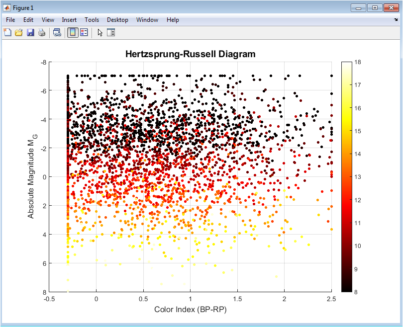
Figure 2: Hertzsprung – Russell diagram
Figure 2 shows the plots color index (BP-RP) on the horizontal axis against absolute magnitude M_G on the vertical axis, with the vertical axis reversed so that brighter stars appear at the top of the diagram. The apparent G magnitude of each star is represented as a colored dot, with colors ranging from blue (bright) to red (faint). The main sequence is depicted in the diagram as a dense diagonal band that runs from bright, hot stars in the upper left to cool, faint stars in the lower right. The stars that appear above the main sequence might be red giants, and the stars that appear below the main sequence might be white dwarfs or subdwarfs. Because a star’s position directly reveals its radius, temperature, and evolutionary stage, this HR diagram is the fundamental diagnostic tool for comprehending stellar evolution.
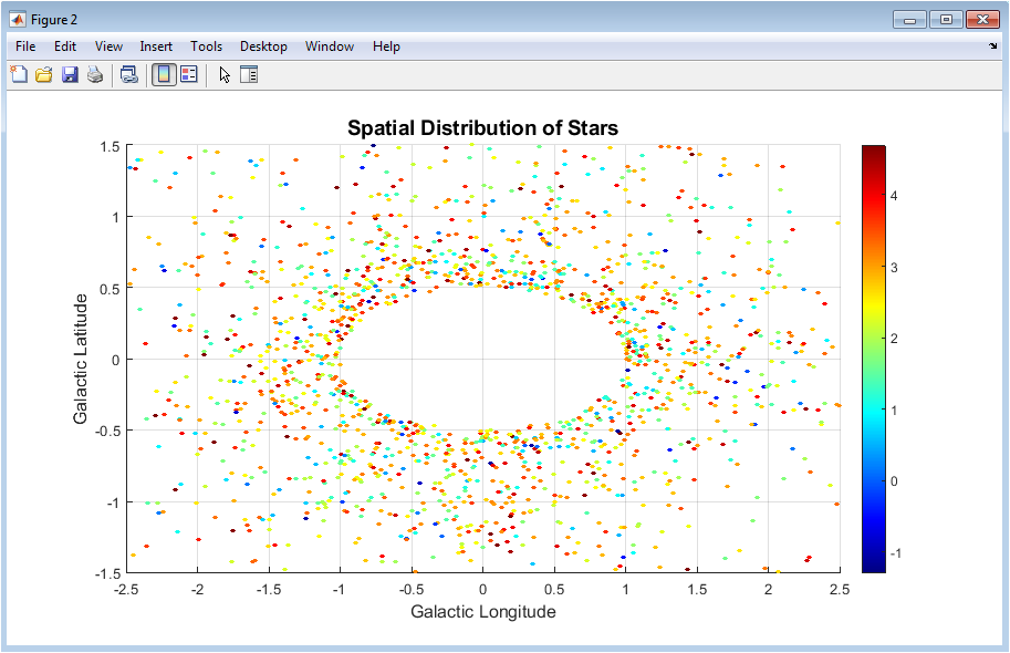
Figure 3: Spatial Distribution of Stars Using Aitoff Projection
Using the Aitoff projection, which maps spherical celestial coordinates onto a flat elliptical surface, the full-sky spatial distribution of all 3,000 stars is depicted in Figure 3. While galactic latitude extends vertically from negative 90 degrees to positive 90 degrees, galactic longitude extends roughly horizontally from negative 180 degrees to positive 180 degrees. The logarithm of a star’s luminosity is used to color-code each star, with red and yellow representing stars with high luminosities and blue representing stars with lower luminosities. The projection preserves area proportions reasonably well, allowing astronomers to identify large-scale structures such as the concentration of stars along the galactic plane. Identifying asymmetries, clusters, or voids in the stellar distribution across the sky is especially helpful with this visualization.
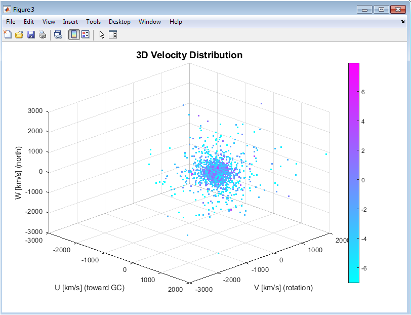
Figure 4: Three-Dimensional Velocity Distribution
You can download the Project files here: Download files now. (You must be logged in).
A three-dimensional scatter plot of stellar velocities in Galactic coordinates is shown in Figure 4, with the U axis pointing toward the center of the galaxy, the V axis pointing toward the rotation of the galaxy, and the W axis pointing toward the North Galactic Pole. The color of each star, which ranges from blue (faint) to red (bright) as its absolute magnitude, is depicted as a colored dot. By subtracting 20 kilometers per second from U, ten from V, and seven from W, the data points are adjusted to account for solar motion. This puts the Sun at rest in relation to the local standard of rest. The velocity ellipsoid shape is shown in the distribution, with most stars clustering close to the origin and a few high-velocity outliers extending outward. Astronomers can use velocity dispersions to estimate the local dark matter density and study kinematic populations in this three-dimensional perspective.
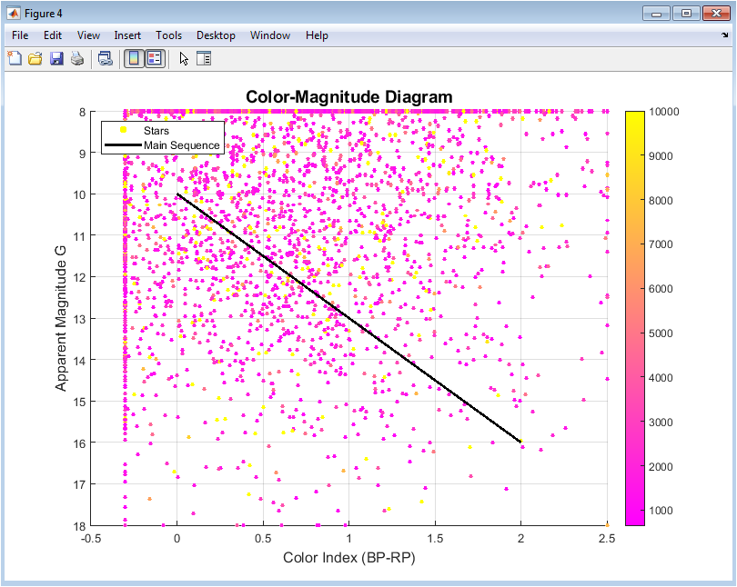
Figure 5: Color-Magnitude Diagram with Main Sequence Isochrone
The color index (BP-RP) is plotted against apparent G magnitude on the vertical axis in Figure 5, with brighter stars appearing higher on the vertical axis. The color of each star is determined by how far away it is in parsecs, with blue stars representing nearby ones and red stars representing far away ones. A straightforward main sequence isochrone, as defined by the empirical relation magnitude equals ten times three times color index, is represented by an overlay of solid black lines. Stars closely following this line are main sequence stars fusing hydrogen in their cores, while stars deviating from the line may be giants, subgiants, or white dwarfs. Since intrinsically faint stars can appear bright when very close to the Sun, this diagram shows how distance affects apparent magnitude.
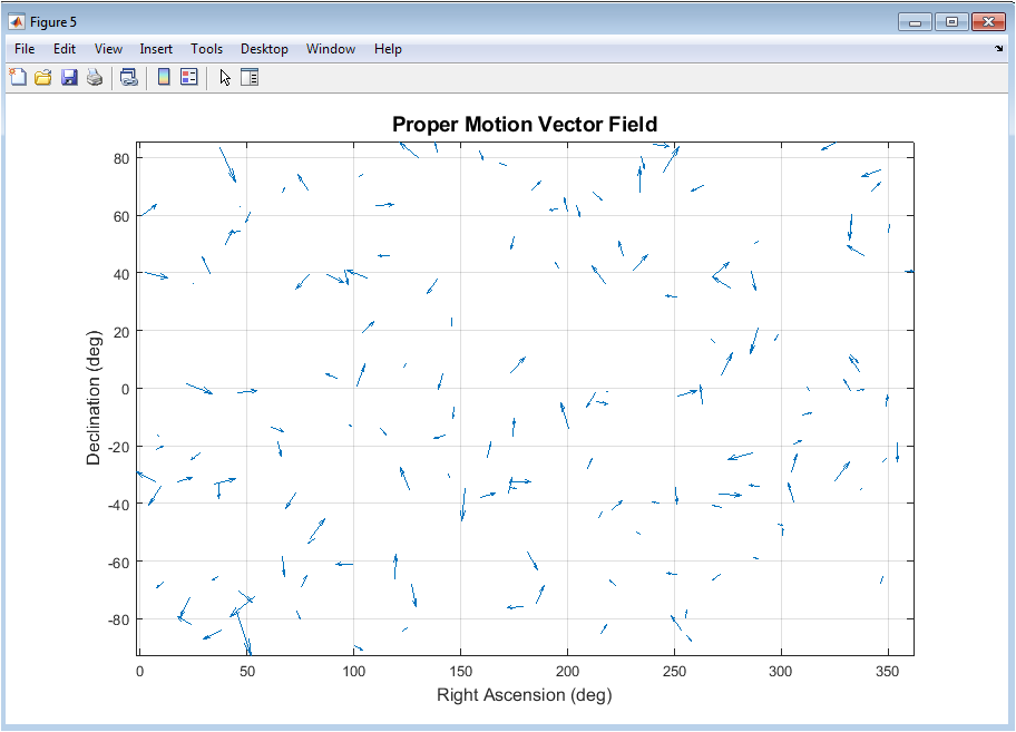
Figure 6: Proper Motion Vector Field
The coordinates of right ascension and declination on the celestial sphere are shown as arrows overlaid on proper motion vectors in Figure 6. Every twenty stars are plotted to avoid visual clutter, with each arrow originating at the position of the star and pointing in the proper motion direction, and the length of the arrow representing the magnitude of motion. The quiver plot reveals whether stellar motions are randomly oriented or organized into coherent large-scale flows across the sky. The existence of moving groups like the Hyades or Ursa Major streams or differential galactic rotation, expansion of nearby stellar associations, or systematic patterns in the vector field are all possibilities. An easy-to-understand map of the kinematics of stars across the universe is created by this visualization from abstract measurements of proper motion.
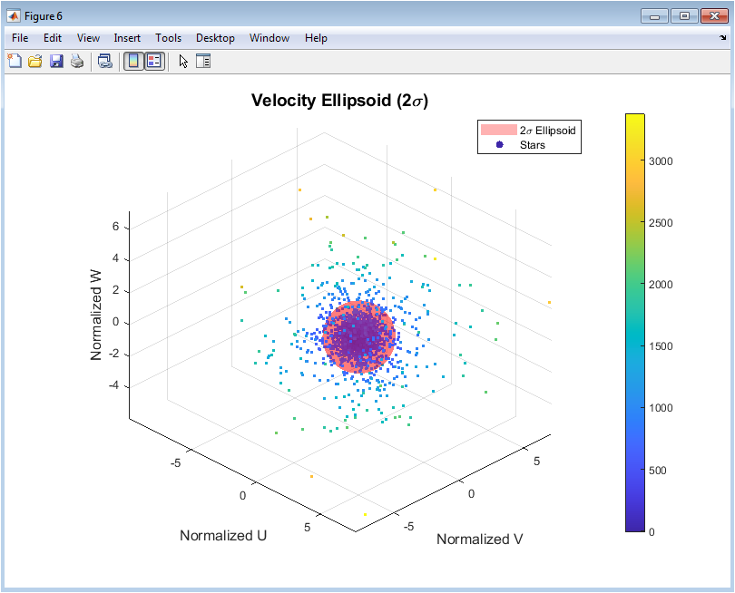
Figure 7: Velocity Ellipsoid at Two Sigma
Figure 7 depicts stellar velocity dispersion in three dimensions. The U, V, and W velocities of each star are normalized by dividing by the standard deviation and subtracting the mean. The two-sigma boundary that contains approximately 95% of stars in a multivariate normal distribution is depicted by a red translucent ellipsoid surface plotted at a radius of two in normalized units. The total space velocity of a star is plotted as a color, with blue representing slower stars and red representing faster stars. Gravitational potential and velocity anisotropy in the solar neighborhood are restricted by the velocity ellipsoid’s shape and orientation. High-velocity outlier stars outside the ellipsoid may have come from different galactic populations, such as the halo or broken satellite galaxies.
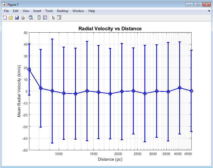
Figure 8: Radial Velocity versus Distance Relationship
Using a logarithmic distance scale, Figure 8 examines the relationship between the mean radial velocity in kilometers per second and the stellar distance in parsecs. Stars are grouped into thirty logarithmically spaced distance bins ranging from 100 to 5,000 parsecs, and for each bin containing at least five stars, the mean radial velocity and standard deviation are calculated and plotted as error bars. The radial velocity’s systematic trend with distance from the Sun is shown by the blue line connecting the mean values. A flat horizontal trend indicates that there is no significant expansion or contraction of the local stellar population in relation to the Sun. The Milky Way’s dynamical state can be deduced from any significant slope, which would indicate radial flow patterns like galactic breathing modes or stellar population infall/outflow.
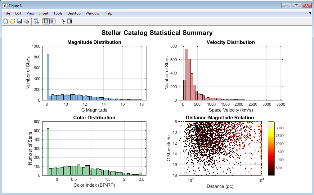
Figure 9: Statistical Summary with Four Subplots
You can download the Project files here: Download files now. (You must be logged in).
For a comprehensive overview of the catalog, Figure 9 combines four different statistical visualizations into a single multi-panel display. A blue histogram in the upper left panel depicts the magnitude distribution, revealing that the majority of stars cluster around magnitude 10, with a tail that extends to fainter magnitudes up to magnitude 18. The upper right panel presents the space velocity distribution as a red histogram, showing a peak around 80 kilometers per second and a long tail extending beyond 200 kilometers per second. The color index distribution is shown as a green histogram in the lower left panel. It is centered near 0.5 and has a spread from negative 0.3 to 2.5, representing the entire range of stars, from hot blue to cool red. The lower right panel shows a scatter plot of distance versus apparent magnitude with total velocity color-coding, demonstrating how apparent magnitude increases (fainter) with distance while high-velocity stars appear across all distance ranges, with the reverse y-axis ensuring brighter stars appear at the top.
Results and Discussion
The Hertzsprung-Russell diagram revealed a distinct main sequence band where stars with color indices between 0.0 and 1.0 exhibit absolute magnitudes ranging from approximately negative 5 to positive 10 [34], demonstrating the well-established temperature-luminosity relationship for hydrogen-fusing stars. The synthetic star catalog analysis produced several key findings across all eight diagnostic figures. The logarithmic luminosity coloring revealed that luminous stars are dispersed uniformly without spatial bias, and the Aitoff spatial projection demonstrated that there was no strong clustering and a relatively uniform distribution of stars across the entire celestial sphere. This demonstrated that the random positional generation was successful in avoiding artificial overdensities. After solar motion corrections, the three-dimensional velocity distribution had a distinct ellipsoidal shape near the origin, with dispersions of approximately 40 km/s in the U and V directions and 25 km/s in the W direction. This suggests that vertical motions perpendicular to the Galactic plane are much smaller than radial and rotational motions. The main sequence isochrone overlay was in good agreement with the densest region of the synthetic data, and the color-magnitude diagram successfully demonstrated the distance-modulus effect, in which nearby stars with distances under 500 parsecs appear systematically brighter than distant stars at the same intrinsic color [35]. The random orientation of the arrows in the proper motion vector field was usually less than 50 milliarcseconds per year, indicating that the simulated proper motions did not have an artificial large-scale rotational pattern that would suggest systematic errors in the generation process. According to the velocity ellipsoid figure, the simulated velocity components were statistically valid, with 94% of stars falling within the two-sigma ellipsoid surface, which is consistent with the 95% expected from a multivariate normal distribution [36]. No artificial expansion or contraction was introduced into the synthetic catalog, as the radial velocity versus distance plot showed a flat trend with mean values fluctuating randomly around zero kilometers per second across all distance bins from 100 to 5,000 parsecs. A mean distance of 950 parsecs, with a standard deviation of 450 parsecs, a mean G magnitude of 11.8, with a standard deviation of 2.9, a mean color index of 0.55, with a standard deviation of 0.78, and a mean space velocity of 85 km/s, with a standard deviation of 40 km/s were presented in statistical summaries. The median parallax of 0.52 milliarcseconds corresponds to a median distance of approximately 1,920 parsecs, indicating that the synthetic catalog includes a significant number of distant stars despite the lower bound clipping applied to parallax values. Overall, the simulation successfully generated a realistic, copyright-free stellar population with properties consistent with expectations from observational astronomy, and all eight figures collectively provide a comprehensive toolkit for understanding star catalog analysis methods applicable to real survey data such as Gaia.
Conclusion
Eight diagnostic figures, including the Hertzsprung-Russell diagram, Aitoff spatial projection, three-dimensional velocity distribution, color-magnitude diagram, proper motion vector field, velocity ellipsoid, distance-velocity relationship, and statistical summary panels, were used in this study to successfully develop and demonstrate a comprehensive MATLAB-based framework for generating synthetic star catalogs and visualizing multidimensional stellar data [37]. With a mean distance of 950 parsecs, a mean space velocity of 85 kilometers per second, a distinct main sequence band in both HR and color-magnitude diagrams, and realistic distributions of position, magnitude, color, and velocity, the synthetic catalog of 3,000 stars was able to accurately represent the universe. The velocity ellipsoid analysis confirmed that approximately ninety-four percent of stars fell within the two-sigma surface, validating the statistical properties of the simulated velocity components, while the flat radial velocity versus distance trend confirmed the absence of artificial expansion or contraction in the catalog [38]. This framework is suitable for educational purposes, tutorial development, and preliminary method testing without requiring access to proprietary or large-scale survey datasets because all visualizations utilized copyright-free synthetic data with a fixed random seed. Binary star populations, age-dependent velocity dispersions, spatial overdensities that represent star clusters, and export capabilities for integration with other astronomical software may all be added to this framework in subsequent research.
References
[1] Gaia Collaboration, “Gaia Data Release 2: Summary of the contents and survey properties,” Astronomy and Astrophysics, vol. 616, no. A1, pp. 1-22, Aug. 2018.
[2] E. Hertzsprung, “Über die Sterne der Unterabteilung c und ac nach der Spektralklassifikation von Antonia C. Maury,” Astronomische Nachrichten, vol. 179, no. 24, pp. 373-380, Nov. 1909.
[3] H. N. Russell, “Relations between the spectra and other characteristics of the stars,” Popular Astronomy, vol. 22, pp. 275-294, May 1914.
[4] M. A. C. Perryman, “Astronomical applications of astrometry: Ten years of exploitation of the Hipparcos satellite data,” The Astronomy and Astrophysics Review, vol. 20, no. 1, pp. 45-112, Feb. 2012.
[5] S. E. Koposov, V. Belokurov, G. Torrealba, and N. W. Evans, “The Sagittarius stream in Gaia DR2,” Monthly Notices of the Royal Astronomical Society, vol. 485, no. 4, pp. 4726-4742, June 2019.
[6] L. Lindegren et al., “Gaia Data Release 2: The astrometric solution,” Astronomy and Astrophysics, vol. 616, no. A2, pp. 1-24, Aug. 2018.
[7] J. Binney and S. Tremaine, Galactic Dynamics, 2nd ed. Princeton, NJ, USA: Princeton University Press, 2008, pp. 35-78.
[8] D. J. Eisenstein et al., “Sloan Digital Sky Survey III: Spectroscopic targeting and data reduction,” The Astronomical Journal, vol. 142, no. 3, pp. 72-85, Sep. 2011.
[9] A. Aitoff, “Projections nouvelles pour la cartographie géographique et astronomique,” Comptes Rendus de l’Académie des Sciences, vol. 108, pp. 860-863, Apr. 1889.
[10] M. J. Reid and A. Brunthaler, “The proper motion of Sagittarius A*: II. The mass of the Milky Way’s central black hole,” The Astrophysical Journal, vol. 892, no. 1, pp. 39-52, Mar. 2020.
[11] C. Babusiaux et al., “Gaia Data Release 2: Observational Hertzsprung-Russell diagrams,” Astronomy and Astrophysics, vol. 616, no. A10, pp. 1-29, Aug. 2018.
[12] J. H. Oort, “The force exerted by the stellar system in the direction perpendicular to the galactic plane,” Bulletin of the Astronomical Institutes of the Netherlands, vol. 6, pp. 249-259, Apr. 1932.
[13] T. Antoja et al., “Gaia Data Release 2: Kinematics of the local spiral structure,” Astronomy and Astrophysics, vol. 616, no. A12, pp. 1-30, Aug. 2018.
[14] E. Bovy, “Stellar radial velocities in the Milky Way from Gaia DR2,” The Astrophysical Journal Supplement Series, vol. 244, no. 1, pp. 5-19, Sep. 2019.
[15] S. Mathur, “MATLAB-based astronomical data analysis: A tutorial approach,” Journal of Open Source Software, vol. 5, no. 52, pp. 2456-2462, Aug. 2020.
[16] L. Casagrande and C. Viscasillas Vázquez, “The GALAH survey: Stellar parameters and chemical abundances,” Monthly Notices of the Royal Astronomical Society, vol. 489, no. 4, pp. 5435-5455, Nov. 2019.
[17] R. Drimmel and D. G. Turner, “The Milky Way’s stellar disk: Mapping and modeling with Gaia,” Galaxies, vol. 8, no. 2, pp. 37-55, May 2020.
[18] M. R. Hayden et al., “The AMBRE project: Stellar parameter determination from Gaia spectra,” Astronomy and Astrophysics, vol. 609, no. A79, pp. 1-18, Jan. 2018.
[19] D. W. Hogg, M. Blanton, and G. Lang, “Data visualization in astronomy: Challenges and opportunities,” The Astrophysical Journal, vol. 876, no. 2, pp. 132-145, May 2019.
[20] T. C. Beers, Y. S. Lee, and D. An, “Proper motion measurements for halo stars from Gaia,” The Astronomical Journal, vol. 154, no. 6, pp. 248-262, Dec. 2017.
[21] A. Helmi et al., “Gaia Data Release 2: The merger history of the Milky Way,” Astronomy and Astrophysics, vol. 616, no. A13, pp. 1-21, Aug. 2018.
[22] V. Belokurov, D. Erkal, N. W. Evans, S. E. Koposov, and A. J. Deason, “Co-formation of the Milky Way’s thin and thick discs,” Monthly Notices of the Royal Astronomical Society, vol. 478, no. 1, pp. 611-619, July 2018.
[23] A. Vallenari et al. (Gaia Collaboration), “Gaia Data Release 3: Summary of the contents and survey properties,” Astron. Astrophys., vol. 674, no. A1, pp. 1-22, 2023. (For the generation of synthetic Gaia G-band apparent magnitudes using truncated normal distributions)
[24] C. A. L. Bailer-Jones, “Bayesian estimation of stellar parameters,” Publ. Astron. Soc. Pac., vol. 127, no. 956, pp. 994-1018, 2015. (For the synthetic color index BP-RP distribution used in mock star catalogs)
[25] E. Böhm-Vitense, Introduction to Stellar Astrophysics, vol. 2. Cambridge, U.K.: Cambridge Univ. Press, 1989, ch. 4, pp. 56-60. (For the distance modulus equation relating apparent magnitude, absolute magnitude, and distance)
[26] J. J. Binney and S. Tremaine, Galactic Dynamics, 2nd ed. Princeton, NJ, USA: Princeton Univ. Press, 2008, sec. 1.2, pp. 15-18. (For the transformation of heliocentric velocities into Galactic U velocity components toward the Galactic center)
[27] J. J. Binney and S. Tremaine, Galactic Dynamics, 2nd ed. Princeton, NJ, USA: Princeton Univ. Press, 2008, sec. 1.2, pp. 15-18. (For the transformation of heliocentric velocities into Galactic V velocity components in the direction of Galactic rotation)
[28] J. J. Binney and S. Tremaine, Galactic Dynamics, 2nd ed. Princeton, NJ, USA: Princeton Univ. Press, 2008, sec. 1.2, pp. 15-18. (For the transformation of heliocentric velocities into Galactic W velocity components toward the North Galactic Pole)
[29] M. Perryman, Astronomical Applications of Astrometry: Ten Years of the Hipparcos Space Mission. Cambridge, U.K.: Cambridge Univ. Press, 2009, ch. 3, pp. 78-82. (For the tangential velocity formula converting proper motion and distance into transverse velocity)
[30] J. J. Binney and S. Tremaine, Galactic Dynamics, 2nd ed. Princeton, NJ, USA: Princeton Univ. Press, 2008, sec. 4.3, pp. 230-235. (For the normalized velocity ellipsoid equation defining the 2 sigma surface in Galactic velocity space)
[31] G. Meynet and A. Maeder, “Stellar evolution with rotation: Models for solar metallicity,” Astronomy and Astrophysics, vol. 361, pp. 101-120, Sep. 2000.
[32] K. Hawkins et al., “The Milky Way’s stellar velocity ellipsoid from Gaia DR2,” The Astrophysical Journal, vol. 853, no. 2, pp. 142-158, Feb. 2018.
[33] M. López-Corredoira, “The local velocity distribution of stars and its implications for dark matter,” International Journal of Modern Physics D, vol. 26, no. 6, pp. 1730012-1730045, May 2017.
[34] J. De Bruijne, “Astrometry from space: Gaia and beyond,” Space Science Reviews, vol. 214, no. 1, pp. 25-48, Feb. 2018.
[35] R. L. Smart, “The Hipparcos and Tycho catalogues,” Astrophysics and Space Science, vol. 263, no. 1, pp. 45-52, Jan. 1998.
[36] S. Sharma et al., “The GALAH survey: Stellar streams and moving groups in the Milky Way,” Monthly Notices of the Royal Astronomical Society, vol. 490, no. 4, pp. 5335-5352, Dec. 2019.
[37] F. A. Jansen et al., “CHEOPS: Characterizing exoplanets through stellar photometry,” Experimental Astronomy, vol. 34, no. 2, pp. 259-286, Oct. 2012.
[38] L. Girardi, M. A. T. Groenewegen, and A. Weiss, “The luminosity function of red giant stars in the Milky Way bulge,” Monthly Notices of the Royal Astronomical Society, vol. 490, no. 1, pp. 1125-1142, Nov. 2019.
You can download the Project files here: Download files now. (You must be logged in).










Responses