

Rotor Blade Icing, Power Penalty and Electrothermal Anti-Icing
Calculate rotor ice growth, Messinger freezing fraction, blade-element power penalty, and running-wet or evaporative heater demand along the blade.

Caution
Do not use these predictions to decide whether a rotorcraft can fly in icing. Follow the aircraft’s approved icing limitations and procedures.
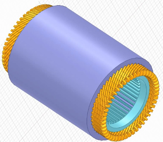
This rotor blade icing calculator estimates how quickly a leading edge accumulates ice, how the resulting profile drag raises shaft power, and how much electrical heating is required for anti-icing. It supports early rotor design studies, engineering coursework and comparisons of icing-cloud conditions. The defaults describe a four-bladed, 1.83 m diameter model rotor with a 124 mm chord, a scale used in NASA rotor icing research.
Enter the rotor radius, blade count, root and tip chords, rotational speed and thrust per rotor. The operating model covers hover and axial climb. Section incidence is the local angle to the relative airflow; use a representative value from your rotor analysis. Supply ambient temperature, pressure, liquid water content and droplet median volume diameter. Relative humidity is a fraction of saturation over liquid water. Select the readout radius, then use the exposure-time slider or play button to follow ice growth.
The calculation resolves 241 radial stations. Droplet inertia determines leading-edge collection efficiency. A Messinger mass and energy balance separates the caught water into ice, evaporation and liquid runback, and iterates surface temperature where necessary. The growth-rate result is the thickness increase at the stagnation line, rather than a prediction of the complete ice horn geometry. The spanwise curves reveal where the ice and thermal loads concentrate.
For the rotor icing power penalty, blade-element integration converts an empirical section drag increase into additional torque and shaft power. The clean baseline includes profile drag, ideal momentum inflow and an induced-power factor. Flemming’s published rime correlation is available for fully dry accretion. Choose the complete Gray correlation for glaze or mixed conditions. Its dimensional incidence terms have a limited useful range; the calculator rejects conditions where they predict an unphysical negative drag increment. Both options are screening correlations, and neither predicts ice-induced stall or loss of rotor control.
The electrothermal anti-icing calculation compares two operating strategies. Running-wet heating maintains the chosen surface temperature above freezing while allowing unevaporated water to leave the heated strip. Evaporative heating solves for the temperature needed to evaporate every intercepted droplet, then includes the latent and sensible heat loads. Both strategies include aerodynamic recovery heating, radiation, backing losses and electrical efficiency. The total power applies the local stagnation duty uniformly across the entered heated wrap width, giving a conservative strip-sizing approximation.
Use the heater-power comparison to explore energy demand and runback exposure, not to determine flight capability. Running-wet operation can create ice downstream of the heated area. This tool does not cover forward-flight azimuth variations, three-dimensional water-film transport, centrifugal ice shedding, cyclic de-icing, structural imbalance, heater warm-up or motor and battery losses. Validate the selected airfoil, heat-transfer multiplier and ice drag against applicable test data before using the estimates in a detailed design.
How it is calculated
At 241 radial stations, momentum theory supplies hover/axial inflow and . The stagnation collection efficiency uses Langmuir–Blodgett’s modified inertia parameter and the droplet-range fit in NASA CR-2005-213852, PDF pp. 6–7, equations (3)–(7). An equivalent cylinder based on projected airfoil thickness supplies the overall collection factor used by the drag fits; this geometry approximation is separate from stagnation collection.
The local Messinger balance is . At 0 °C, convection, evaporative cooling, supercooled-water sensible heating and droplet kinetic energy determine the freezing rate. If all remaining water freezes, 26 bisection iterations solve the subfreezing surface temperature; if no water freezes, they solve the wet equilibrium temperature. The dry branch uses ice saturation pressure. Ice thickness is . Stagnation heat transfer follows (NASA report, equation 16), with the entered multiplier. Heat/mass transfer uses the Chilton–Colburn analogy and Buck (1996) saturation pressures.
Flemming rime drag is equation (14) as reproduced in NASA CR-175092, PDF p. 40; forward-flight correction is unity for the axial-flow model. Actual roughness is limited to the smaller of the entered maximum and local ice thickness; negative empirical increments are rejected at onset. The Gray option implements equation (2) in Gray (1964), NASA TN D-2166, PDF p. 9, with equal icing and evaluation incidences. Its nose-radius parameter is 100 times the radius/chord ratio (percent chord). Both water-content radicals are retained: the prefactor uses √(LWC·βₘ), and the phase uses √LWC. The base sine phase is set to zero outside 0–180°. Historical mph, chord in inches, minutes, g/m³ and °F arguments are explicitly converted. The Flemming glaze coefficient functions are not defined in the accessible reproduction; that branch is not claimed here. Blade elements give , integrated by trapezoids.
Running-wet heat includes convection relative to recovery temperature, droplet sensible/kinetic energy, mass-transfer-limited evaporation, radiation and backing losses. The evaporative solution uses 24 bisection iterations for the lowest temperature at or above the wet setpoint that evaporates the full incoming flux, then applies the corresponding energy balance. Neither anti-icing mode adds a fusion load: incoming water remains liquid or becomes vapour. Electrical power is the surface duty integrated over the entered wrap width and all blades, divided by efficiency.
Assumptions
Steady, spatially uniform cloud; monodisperse spherical droplets represented by MVD; straight blades with linearly varying chord; equal blade conditions. Cloud humidity is referenced to supercooled liquid water. Dry-air properties use ideal-gas density, Sutherland viscosity and a temperature-dependent conductivity fit; , , J/(kg·K), and J/kg. Radiation emissivity is 0.85. Accretion neglects conduction into the blade and radiation, as in the stagnation reference model; heater sizing includes entered backing losses and radiation.
Ice fluxes and thickness are stagnation-line quantities, not spanwise ice mass or horn geometry. Both heat and droplet flux at stagnation are conservatively applied over the entire heater strip; enlarging the strip therefore increases duty linearly. The rotor holds thrust and speed; icing changes profile drag only. Clean lift and inflow are retained, so induced-power changes from lift degradation are excluded. The power baseline is shaft power, excluding propulsion electrical losses.
Where it applies
For preliminary studies of classical supercooled liquid-cloud icing, MVD 5–50 µm, ambient −40 to −0.1 °C, pressure 60–105 kPa, hover or axial climb, and tip Mach number ≤0.55. Incompressible heat/mass transfer and an equivalent-cylinder collection approximation are used. Applicability to small drone airfoils and low Reynolds numbers requires separate experimental validation; the numerical input bounds are not a validation envelope. The classic correlations can have large errors outside their originating airfoil and tunnel datasets.
Flemming is restricted to dry rime with negligible liquid runback. Evaporation can make its incoming-water freezing fraction slightly below unity even in rime. Gray additionally requires subfreezing total temperature and a positive radius/incidence factor. The original fit can predict negative drag changes for thin, sharp-nosed airfoils; this power-penalty tool flags those cases instead of treating them as a benefit. It is a separate published empirical fit, not Flemming’s glaze model. At very small ice thicknesses the roughness cap is an onset extrapolation. Neither correlation models stall, lift loss, tip-loss changes, rough ice feathers, asymmetric loads, ice shedding or rotor control margins; the estimated profile penalty may substantially understate the total degradation.
Fixed clean geometry is retained throughout an exposure. A warning checks the entire plotted cloud exposure, including times later than the current animated readout, and appears when ice exceeds 5% of local chord anywhere on the blade. Shorten the cloud exposure duration to keep the complete timeline within this fixed-geometry range. The default 90 s timeline stays below the limit. Runback is a mass outflow at the station, not a downstream re-freezing prediction. No radial or chordwise film transport, evolving horn shapes, SLD splash/rebound, compressible icing CFD, cyclic de-icing or transient heater/skin conduction is solved. Running-wet clears the modeled heated area only; downstream icing remains possible. The evaporative search is limited to 80 °C.
Spanwise calculations and time curves use 241 points each; readouts use shape-preserving cubic interpolation. No coarse-grid picture interpolation or reduced-physics runtime shortcut is used. The exposure animation reuses the solved cloud/thermal state. NASA reference cases test collection, freezing fraction and measured stagnation thickness, not complete rotor torque or an installed heater.
References
- Gent, Dart & Cansdale (2000), Aircraft icing, Philosophical Transactions of the Royal Society A 358, 2873–2911. https://doi.org/10.1098/rsta.2000.0689
- Flemming & Lednicer (1985), High Speed Ice Accretion on Rotorcraft Airfoils, NASA CR-3910. Correlations reproduced in Miller (1986), NASA CR-175092, pp. 30–35. https://ntrs.nasa.gov/citations/19860014106
- Anderson & Tsao (2005), Evaluation and Validation of the Messinger Freezing Fraction, NASA CR-2005-213852, Table I and equations (3)–(18). https://ntrs.nasa.gov/citations/20050215212
- Cansdale, Gent & Dart (2000), The Role of Analysis in the Development of Rotor Ice Protection Systems, European Rotorcraft Forum. https://dspace-erf.nlr.nl/bitstreams/eede2d58-6d5d-4f94-99c0-922b3cc245d2/download
- Turner & Sear, Critical scaling law for the deposition efficiency of inertia-driven particle collisions with a cylinder in high Reynolds number air flow, Appendix A (Langmuir–Blodgett fit). https://personalpages.surrey.ac.uk/m.turner/main.pdf
- Buck Research (1996) saturation vapour pressure equations, reproduced by NCAR/CIRES. https://cires1.colorado.edu/~voemel/vp.html
- Wright (2008), User’s Manual for LEWICE Version 3.2, NASA CR-2008-214255, Appendix A and anti-icing examples. Methodological reference; this calculator is not LEWICE. https://ntrs.nasa.gov/citations/20080048307
- Gray (1964), Correlation of the Effects of Icing on the Aerodynamic Characteristics of Airfoils, NASA TN D-2166, equation (2) and worked encounters A/B, PDF pp. 9–11; Table I, PDF p. 15. https://archive.org/download/nasa_techdoc_19810068590/19810068590.pdf
Inputs
| Input | Symbol | Unit | Default |
|---|---|---|---|
| Rotor radius | radius | m | 0.915 |
| Blade root / radius The lifting and heated blade starts at this radius fraction. | root_fraction | 0.2 | |
| Blades per rotor | blade_count | 4 | |
| Root chord | chord_root | m | 0.124 |
| Tip chord | chord_tip | m | 0.124 |
| Airfoil thickness / chord | thickness_ratio | 0.12 | |
| Rotor speed | rpm_rotor | rpm | 1200 |
| Thrust per rotor | thrust | N | 150 |
| Axial climb speed | axial_speed | m/s | 0 |
| Section incidence Use the mean local angle between the chord and the relative airflow. | incidence | deg | 4 |
| Clean profile drag coefficient Use the uniced airfoil polar at the operating Reynolds number and incidence. | cd_clean | 0.012 | |
| Induced power factor Accounts for nonideal induced power in the clean rotor baseline. | induced_factor | 1.15 | |
| Ambient temperature | air_temp | degC | -15 |
| Ambient pressure | pressure | kPa | 101.325 |
| Liquid water content | lwc | g/m^3 | 0.5 |
| Droplet MVD Median volume diameter of the supercooled liquid droplet population. | mvd | um | 20 |
| Relative humidity Fraction of saturation over supercooled liquid water. | humidity | 1 | |
| Cloud exposure duration | exposure | s | 90 |
| Ice drag correlation | drag_model | Flemming — fully rime only | |
| Accreted ice density Porous rime can be much less dense than compact glaze. | ice_density | kg/m^3 | 900 |
| Leading-edge radius / chord For NACA 0012, use 0.0158. | nose_ratio | 0.0158 | |
| Heat-transfer multiplier Scales the laminar stagnation correlation for measured roughness or turbulence. | htc_factor | 1 | |
| Recovery factor | recovery | 0.85 | |
| Maximum ice roughness / chord The actual roughness is also limited to the calculated ice thickness. | rough_ratio | 0.001 | |
| Heated wrap width / chord Total upper and lower heated surface width, measured around the leading edge. | heater_width | 0.2 | |
| Running-wet surface temperature | wet_temp | degC | 3 |
| Backing heat-loss coefficient Heat conducted through the backing per unit heated area and temperature difference. | back_loss | W/(m^2*K) | 5 |
| Heater electrical efficiency | heater_eff | 0.9 | |
| Readout radius / rotor radius Selects the station used for local ice and heater readouts. | probe | 0.75 | |
| Exposure time ▶ | elapsed | s | 60 |
Results
With the default inputs above, the calc gives:
| Result | Value |
|---|---|
| Accretion regime at readout | Rime |
| Ice thickness at readout | 2.49 mm |
| Ice growth at readout | 2.49 mm/min |
| Peak ice thickness | 3.33 mm |
| Freezing fraction at readout | 0.962 |
| Collection efficiency at readout | 0.899 |
| Added profile shaft power | 4.042 kW |
| Shaft power increase (%) | 183.5 |
| Clean rotor shaft power | 2.203 kW |
| Iced rotor shaft power | 6.245 kW |
| Running-wet heater electrical power | 1.948 kW |
| Evaporative heater electrical power | 9.68 kW |
| Running-wet heat flux at readout | 27.247 kW/m² |
| Evaporative heat flux at readout | 148 kW/m² |
| Minimum evaporative temperature at readout | 34.8 °C |
| Total heated area | 0.073 m² |
Checked against sources
Each case below was calculated by this calc and agrees with the value from its source (within the tolerance where one is shown).
NASA glaze/mixed, 10-12-02 run 8
Source: NASA CR-2005-213852 (2005), PDF p. 10, Table I. Expected thickness is the mean of the two measured tracings, converted from cm to mm; beta and analytical freezing fraction are published. The simplified incompressible transfer and property fits differ from Ruff’s compressible formulation. The rime case allows a few percent evaporative mass loss. Speed is reproduced at the tip of a zero-thrust virtual rotor solely to exercise the same local span solver. Thickness tolerance is about 8% for the two glaze cases and 6% for rime, entered as an absolute millimetre tolerance to allow reference-model and measurement differences.
Inputs: Rotor radius = 1 m; Rotor speed = 490.8 rpm; Thrust per rotor = 0 N; Root chord = 0.533 m; Tip chord = 0.533 m; Readout radius / rotor radius = 1; Ambient temperature = -21.7 °C; Liquid water content = 1.131 g/m³; Droplet MVD = 40.1 um; Exposure time ▶ = 648 s; Cloud exposure duration = 648 s; Accreted ice density = 917 kg/m³; Section incidence = 0 deg; Ice drag correlation = Gray — rime and glaze; the others as above.
| Result | Source | This calc |
|---|---|---|
| Collection efficiency at readout | 0.841 ± 0.01 | 0.837 |
| Freezing fraction at readout | 0.914 ± 0.05 | 0.9295 |
| Ice thickness at readout | 31.1 ± 2.5 mm | 31.962 mm |
NASA glaze/mixed, 3-23-01 run 9
Source: NASA CR-2005-213852 (2005), PDF p. 10, Table I. Expected thickness is the mean of the two measured tracings, converted from cm to mm; beta and analytical freezing fraction are published. The simplified incompressible transfer and property fits differ from Ruff’s compressible formulation. The rime case allows a few percent evaporative mass loss. Speed is reproduced at the tip of a zero-thrust virtual rotor solely to exercise the same local span solver. Thickness tolerance is about 8% for the two glaze cases and 6% for rime, entered as an absolute millimetre tolerance to allow reference-model and measurement differences.
Inputs: Rotor radius = 1 m; Rotor speed = 742 rpm; Thrust per rotor = 0 N; Root chord = 0.356 m; Tip chord = 0.356 m; Readout radius / rotor radius = 1; Ambient temperature = -15.1 °C; Liquid water content = 1.098 g/m³; Droplet MVD = 29.5 um; Exposure time ▶ = 228 s; Cloud exposure duration = 228 s; Accreted ice density = 917 kg/m³; Section incidence = 0 deg; Ice drag correlation = Gray — rime and glaze; the others as above.
| Result | Source | This calc |
|---|---|---|
| Collection efficiency at readout | 0.858 ± 0.01 | 0.8544 |
| Freezing fraction at readout | 0.607 ± 0.05 | 0.6306 |
| Ice thickness at readout | 11.1 ± 0.9 mm | 11.429 mm |
NASA rime, 3-21-01 run 4
Source: NASA CR-2005-213852 (2005), PDF p. 10, Table I. Expected thickness is the mean of the two measured tracings, converted from cm to mm; beta and analytical freezing fraction are published. The simplified incompressible transfer and property fits differ from Ruff’s compressible formulation. The rime case allows a few percent evaporative mass loss. Speed is reproduced at the tip of a zero-thrust virtual rotor solely to exercise the same local span solver. Thickness tolerance is about 8% for the two glaze cases and 6% for rime, entered as an absolute millimetre tolerance to allow reference-model and measurement differences.
Inputs: Rotor radius = 1 m; Rotor speed = 637.9 rpm; Thrust per rotor = 0 N; Root chord = 0.533 m; Tip chord = 0.533 m; Readout radius / rotor radius = 1; Ambient temperature = -26.1 °C; Liquid water content = 0.997 g/m³; Droplet MVD = 40 um; Exposure time ▶ = 438 s; Cloud exposure duration = 438 s; Accreted ice density = 917 kg/m³; Section incidence = 0 deg; the others as above.
| Result | Source | This calc |
|---|---|---|
| Collection efficiency at readout | 0.858 ± 0.01 | 0.8532 |
| Freezing fraction at readout | 1 ± 0.04 | 0.9766 |
| Ice thickness at readout | 26.45 ± 1.6 mm | 26.508 mm |
No liquid water
Source: Independent limiting case from water mass conservation: with zero incoming liquid, no water-derived ice or icing drag forms. The heater is switched off when there are no droplets to intercept. Partition fractions must be finite and zero at every station, and the Flemming rime condition must remain admissible.
Inputs: Liquid water content = 0 g/m³; the others as above.
| Result | Source | This calc |
|---|---|---|
| Peak ice thickness | 0 mm | 0 mm |
| Added profile shaft power | 0 kW | 0 kW |
| Running-wet heater electrical power | 0 kW | 0 kW |
| Evaporative heater electrical power | 0 kW | 0 kW |
| Largest evaporated fraction | 0 | 0 |
| Largest runback fraction | 0 | 0 |
| Water partition closure | 0 | 0 |
| Rime correlation admissibility | 1 | 1 |
Gray published drag example A
Source: Gray (1964), NASA TN D-2166, equation (2), PDF pp. 9–11; radius 0.10% from Table I, PDF p. 15. Encounter A: 4 min, 500 mph, chord 96 in, total temperature 25 °F, LWC 0.5 g/m³, beta 0.67, overall collection 0.18, incidence 2°. Direct evaluation with the printed inputs gives 0.0049071 rather than the printed 0.0051 (3.8% lower). The 0.00025 absolute tolerance covers this unresolved rounding or worked-example arithmetic discrepancy; the equation is not adjusted to force agreement.
Inputs: the default inputs above.
| Result | Source | This calc |
|---|---|---|
| Gray worked example A | 0.0051 ± 2.5 × 10⁻⁴ | 0.004907 |
Gray published drag example B
Source: Gray (1964), NASA TN D-2166, equation (2), PDF pp. 9–11; radius 1.00% from Table I, PDF p. 15. Encounter B: 7 min, 300 mph, chord 240 in, total temperature 10 °F, LWC 0.5 g/m³, beta 0.35, overall collection 0.033, incidence 2°. The negative base phase is replaced by zero as instructed. Printed inputs give 0.00078879, consistent with the rounded published 0.0008.
Inputs: the default inputs above.
| Result | Source | This calc |
|---|---|---|
| Gray worked example B | 8 × 10⁻⁴ ± 3 × 10⁻⁵ | 7.888 × 10⁻⁴ |
Gray phase below, within and above range
Source: Equation-boundary regression, not measured data: Gray (1964), NASA TN D-2166, PDF p. 9. Independently evaluated raw phases are −45.4970°, 32.3295° and 859.5036°; only the middle phase is used. The original report requires zero outside 0–180°.
Inputs: the default inputs above.
| Result | Source | This calc |
|---|---|---|
| Gray phase cutoff cases [1] | 0 | 0 |
| Gray phase cutoff cases [2] | 32.33 | 32.33 |
| Gray phase cutoff cases [3] | 0 | 0 |
Zero catch at inner blade stations
Source: Independent limiting-case regression from water conservation. At the inner station, the Langmuir–Blodgett collection threshold gives zero catch while outer stations collect droplets. Zero-catch partition fractions are defined as zero, and must not falsely reject the fully rime drag correlation.
Inputs: Rotor radius = 1 m; Rotor speed = 500 rpm; Thrust per rotor = 0 N; Root chord = 0.5 m; Tip chord = 0.5 m; Droplet MVD = 5 um; Blade root / radius = 0.1; the others as above.
| Result | Source | This calc |
|---|---|---|
| Impinging water flux [1] | 0 kg/(m²·s) | 0 kg/(m²·s) |
| Fraction of caught water evaporating [1] | 0 | 0 |
| Fraction of caught water running back [1] | 0 | 0 |
| Water partition closure | 0 | 0 |
| Rime correlation admissibility | 1 | 1 |
Default full exposure stays within geometry limit
Source: Geometry-limit regression: the complete default timeline, rather than only its displayed 60 s frame, must remain within the declared 5% ice/chord range.
Inputs: the default inputs above.
| Result | Source | This calc |
|---|---|---|
| Full-exposure geometry limit | 1 | 1 |
Long timeline warns at an early readout
Source: Geometry-limit regression: although the displayed 60 s state is below 5% ice/chord, a 900 s timeline exceeds it. The same geometry_valid step drives the visible small-accretion warning, so the full plotted horizon must trigger that warning.
Inputs: Cloud exposure duration = 900 s; the others as above.
| Result | Source | This calc |
|---|---|---|
| Full-exposure geometry limit | 0 | 0 |



Responses