

Four-Bar Linkage Calculator and Coupler Curve Analyzer
Analyze Grashof type, link positions, velocities, accelerations, and transmission angle. Animate either assembly branch and trace a coupler curve.

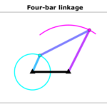
This four bar linkage calculator helps mechanism students, engineers, and makers explore a planar mechanism before building a prototype. Enter four pin-to-pin lengths to see whether the linkage satisfies the Grashof condition, inspect its instantaneous motion, and watch a point fixed to the coupler draw its coupler curve. The default dimensions describe a crank–rocker with a 100 mm ground link and a 40 mm input link.
Start with the ground distance O₂–O₄, input link O₂–A, coupler A–B, and output link O₄–B. The ground lies along the positive horizontal axis. All link angles are measured counterclockwise from that axis, and positive angular velocity or acceleration means counterclockwise motion. The metric/US control converts physical inputs and result cards; chart axes and the point tables explicitly retain their stated calculation units.
Choose an assembly branch and move the input-angle slider, or press play to preview a revolution. The plus branch locates B to the left of the directed line from A to O₄; the minus branch selects the other circle intersection. They correspond to open and crossed configurations at the defaults, but those names are not reliable throughout every mechanism’s motion. Playback sweeps angle for inspection: its speed and direction do not simulate the entered angular velocity or acceleration. A limited-motion mechanism stops playing when it reaches an unreachable or singular pose.
Define point P by its distance AP and its counterclockwise offset β from the coupler direction A–B. The colored curve shows P’s reachable path for the selected branch; the moving dot identifies the current point. Set AP to zero to track A, or set AP equal to the coupler length with β equal to zero to track B. Impossible parts of an angle sweep appear as gaps, rather than connecting through an unavailable configuration.
The result cards report link angles, angular rates, angular accelerations, the transmission angle, and P’s motion. The point tables provide signed horizontal and vertical components for A, B, and P. The transmission angle is the acute angle between the coupler and output link: approaching zero indicates a toggle and increasing sensitivity. Its reported minimum covers all geometrically reachable input angles, including limiting positions, rather than only the sampled chart points.
Grashof classification describes rotational capability, not strength or satisfactory force transmission. Equality is a change-point mechanism that can switch branches at a collinear pose. This analyzer assumes rigid links and ideal pins. It does not calculate drive torque, bearing reactions, friction, backlash, flexibility, collision clearance, or fatigue. Use the kinematic results as inputs to a separate load and strength analysis before selecting a motor or manufacturing a mechanism.
How it is calculated
The position solution uses the two circle constraints |AB| = L₃ and |O₄B| = L₄. With d = O₄ − A, q = |d|, u = (L₃² − L₄² + q²)/(2q), and h = √(L₃² − u²), B = A + u d/q + σ h (−dᵧ,dₓ)/q. The branch sign σ is +1 or −1. atan2 determines each link angle in the correct quadrant, displayed in 0°…360°.
The velocity loop is L₂ω₂(−sin θ₂, cos θ₂) + L₃ω₃(−sin θ₃, cos θ₃) = L₄ω₄(−sin θ₄, cos θ₄). Its two scalar equations determine ω₃ and ω₄. Differentiating again adds the centripetal terms −ω²r and gives a second two-equation solve for α₃ and α₄. Point P then uses vP = vA + ω₃ × AP and aP = aA + α₃ × AP − ω₃² AP.
Grashof margin is (P + Q) − (S + L), using the sorted lengths. Positive means strict Grashof; zero within a relative roundoff tolerance means a change point. The shortest link's relation to the selected ground determines the inversion. Acute transmission angle is acos(|cos(θ₄ − θ₃)|). Its exact minimum follows from the endpoints of the reachable A–O₄ separation interval. Reachable input intervals are [θlow, θhigh] and [360° − θhigh, 360° − θlow]; exclude singular endpoints when solving rates.
Method sources: Williams, Ohio University ME 3011 notes, pp. 23–25 (loop closure and branches), 39–40 (Grashof), 61–63 (velocity), and 78–81 (acceleration); University of Almería, worked example 2.1 (circle construction and point kinematics). The sweep uses 241 positions at 1.5° spacing. Curve segmentation is cached independently of the playing angle.
When forming linear motion, angular derivatives are normalized by one radian, treating the radian as dimensionless in SI. The small residuals used solely for closure verification are rounded at 10⁻¹² relative length, 10⁻⁹ mm/s, and 10⁻⁸ mm/s² to suppress floating-point cancellation; computed motion retains full precision.
The drawing envelope uses only reachable sweep coordinates, the fixed pivots, and the current reachable pose. Unreachable circle-intersection constructions are excluded from both the plotted path and the viewport bounds.
Assumptions
- Planar, rigid, constant-length links with four ideal revolute joints; the ground is fixed.
- P is fixed to the coupler; AP and β describe a rigid offset, including an extension beyond the physical bar.
- Angular velocity and angular acceleration are instantaneous prescribed values. The angular-rate chart holds the specified ω₂ constant while varying pose.
- Crossing links may occupy parallel planes; geometric interference is not tested.
- Length inputs share a common calculation unit of mm. Formula and chart units remain as labeled when result cards are converted to US units.
Where it applies
Use positive link lengths and a longest link shorter than the sum of the other three. The selected angle must satisfy |L₃ − L₄| ≤ |A O₄| ≤ L₃ + L₄. A coincident A and O₄ gives no unique circle-intersection construction.
At |sin(θ₃ − θ₄)| ≤ 10⁻⁶ the velocity matrix is singular or numerically ill-conditioned, so instantaneous rate results are withheld. A warning is shown below a 5° transmission angle; this is a sensitivity notice, not an acceptance criterion. Change-point chains can jump branches and require an external constraint to select their passage through collinearity. Roundoff guards do not make an unreachable pose valid.
This is kinematics only: no forces, motor sizing, elastic deformation, joint clearance, losses, or structural safety prediction. Sweeps sample the curve and may miss a very narrow reachable interval; the reported angle limits and minimum transmission angle are analytical.
References
- R. L. Williams II, ME 3011 Kinematics and Dynamics of Machines, Ohio University, pp. 23–25, 39–40, 60–63, 78–82. Open course notes: https://people.ohio.edu/williams/html/PDF/NotesBook3011.pdf
- Mechanical Engineering, University of Almería, Machine and Mechanism Theory, Example 2.1: Kinematic analysis of a four-bar linkage. https://ingmec.ual.es/tmm/L02_05_example1.html
- SoftIntegration, Ch Mechanism Toolkit, version 3.0 (2015), CFourbar::angularAccel example, printed pp. 241–243 (PDF pp. 250–252). https://www.softintegration.com/download/software/release/docs/chmechanism.pdf
- Robert L. Norton, Design of Machinery, 6th edition, McGraw-Hill. Background reading on linkage position, velocity, acceleration, and coupler curves; author site: https://designofmachinery.com/
- J. J. Uicker Jr., G. R. Pennock, and J. E. Shigley, Theory of Machines and Mechanisms, 6th edition, Cambridge University Press (2023). Background reading: https://doi.org/10.1017/9781009303644
Inputs
| Input | Symbol | Unit | Default |
|---|---|---|---|
| Ground length L₁ · O₂–O₄ | L_1 | mm | 100 |
| Input length L₂ · O₂–A | L_2 | mm | 40 |
| Coupler length L₃ · A–B | L_3 | mm | 120 |
| Output length L₄ · O₄–B | L_4 | mm | 80 |
| Input angle θ₂ · ▶ preview Measured counterclockwise from the ground line O₂ → O₄. Play sweeps the angle at a display speed independent of the specified input rate; it stops at an unreachable or singular position. | theta_2 | deg | 40 |
| Assembly branch The + branch places B to the left of the directed line A → O₄ (positive signed cross product); the − branch places it to the right. These signs stay unambiguous through a revolution. | assembly | + branch · open at defaults | |
| Input angular velocity ω₂ Positive is counterclockwise; negative is clockwise. This is the instantaneous rate used for kinematics, not the animation playback speed. | omega_2 | rad/s | 25 |
| Input angular acceleration α₂ Instantaneous signed acceleration. Use zero for constant input speed. | alpha_2 | rad/s^2 | 15 |
| Coupler point distance AP P is fixed to the coupler; AP may extend beyond the link. Set AP = 0 to follow joint A. | r_AP | mm | 90 |
| Coupler point offset angle β Counterclockwise from A → B to A → P. Use β = 0° and AP = L₃ to follow joint B. | beta_P | deg | 40 |
Results
With the default inputs above, the calc gives:
| Result | Value |
|---|---|
| Grashof classification | Grashof · crank–rocker |
| Input motion | Full revolution · no toggle |
| Grashof margin | 20 mm |
| Coupler angle θ₃ | 20.298 deg |
| Output angle θ₄ | 57.325 deg |
| Transmission angle μ | 37.027 deg |
| Minimum reachable transmission angle | 26.384 deg |
| Coupler angular velocity ω₃ | -4.1209 rad/s |
| Output angular velocity ω₄ | 6.998 rad/s |
| Coupler angular acceleration α₃ | 296.089 rad/s² |
| Output angular acceleration α₄ | 470.134 rad/s² |
| Coupler point x | 75.236 mm |
| Coupler point y | 103.887 mm |
| Coupler point speed | 664.719 mm/s |
| Coupler point acceleration | 43,601.073 mm/s² |
Checked against sources
Each case below was calculated by this calc and agrees with the value from its source (within the tolerance where one is shown).
University of Almería · position and acceleration
Source: University of Almería, Machine and Mechanism Theory, Example 2.1, numerical position, velocity, and acceleration sections: https://ingmec.ual.es/tmm/L02_05_example1.html . Lengths converted from m to mm; source point C is this tool's P. The source rounds A and link vectors to 0.001 m before velocity calculations: it reports ω₃ = 0.328 and ω₄ = 0.821, while full-precision geometry gives 0.329296 and 0.823078 rad/s. The correct unrounded kinematics are retained; component tolerances allow the published rounding.
Inputs: Ground length L₁ · O₂–O₄ = 500 mm; Input length L₂ · O₂–A = 200 mm; Coupler length L₃ · A–B = 600 mm; Output length L₄ · O₄–B = 500 mm; Input angle θ₂ · ▶ preview = 135 deg; Input angular velocity ω₂ = 2 rad/s; Input angular acceleration α₂ = -1.5 rad/s²; Coupler point distance AP = 400 mm; Coupler point offset angle β = 30 deg; the others as above.
| Result | Source | This calc |
|---|---|---|
| Coupler angle θ₃ | 34.18 deg | 34.18 deg |
| Output angle θ₄ | 106.9 deg | 106.9 deg |
| Coupler point x | 32.8 ± 0.1 mm | 32.798 mm |
| Coupler point y | 501.5 mm | 501.5 mm |
| Coupler angular acceleration α₃ | 0.427 ± 0.002 rad/s² | 0.4271 rad/s² |
| Output angular acceleration α₄ | -1.007 ± 0.002 rad/s² | -1.007 rad/s² |
| Coupler point P · x acceleration | 605 ± 1 mm/s² | 605.1 mm/s² |
| Coupler point P · y acceleration | -318 ± 1 mm/s² | -318.2 mm/s² |
| Coupler point P · x velocity | -400 ± 2 mm/s | -401.4 mm/s |
| Coupler point P · y velocity | -225 ± 1 mm/s | -225.5 mm/s |
Ch Mechanism Toolkit · circuit 1 angular accelerations
Source: SoftIntegration, Ch Mechanism Toolkit v3.0 (2015), CFourbar::angularAccel, printed pp. 241–243; PDF pp. 250–252. Circuit 1 output: alpha3=4.0181, alpha4=-9.7407 rad/s². Original dimensions in m converted to mm. https://www.softintegration.com/download/software/release/docs/chmechanism.pdf
Inputs: Ground length L₁ · O₂–O₄ = 12,000 mm; Input length L₂ · O₂–A = 4,000 mm; Coupler length L₃ · A–B = 12,000 mm; Output length L₄ · O₄–B = 7,000 mm; Input angle θ₂ · ▶ preview = 150 deg; Input angular velocity ω₂ = 5 rad/s; Input angular acceleration α₂ = -5 rad/s²; Coupler point distance AP = 0 mm; Coupler point offset angle β = 0 deg; the others as above.
| Result | Source | This calc |
|---|---|---|
| Coupler angular acceleration α₃ | 4.018 rad/s² | 4.018 rad/s² |
| Output angular acceleration α₄ | -9.741 rad/s² | -9.741 rad/s² |
Ch Mechanism Toolkit · circuit 2 angular accelerations
Source: SoftIntegration, Ch Mechanism Toolkit v3.0 (2015), CFourbar::angularAccel, printed pp. 241–243; PDF pp. 250–252. Circuit 2 output: alpha3=-3.7875, alpha4=9.9712 rad/s². Original dimensions in m converted to mm. https://www.softintegration.com/download/software/release/docs/chmechanism.pdf
Inputs: Ground length L₁ · O₂–O₄ = 12,000 mm; Input length L₂ · O₂–A = 4,000 mm; Coupler length L₃ · A–B = 12,000 mm; Output length L₄ · O₄–B = 7,000 mm; Input angle θ₂ · ▶ preview = 150 deg; Input angular velocity ω₂ = 5 rad/s; Input angular acceleration α₂ = -5 rad/s²; Coupler point distance AP = 0 mm; Coupler point offset angle β = 0 deg; Assembly branch = − branch · crossed at defaults; the others as above.
| Result | Source | This calc |
|---|---|---|
| Coupler angular acceleration α₃ | -3.788 rad/s² | -3.788 rad/s² |
| Output angular acceleration α₄ | 9.971 rad/s² | 9.971 rad/s² |
Ohio University · strict Grashof example
Source: R. L. Williams II, Ohio University ME 3011 notes, p. 40, Grashof's Law Examples, example 1. The published dimension ratios give margin (8 + 7) − (10 + 4) = 1. The common length scale is arbitrary; mm are used here. https://people.ohio.edu/williams/html/PDF/NotesBook3011.pdf
Inputs: Ground length L₁ · O₂–O₄ = 10 mm; Input length L₂ · O₂–A = 4 mm; Coupler length L₃ · A–B = 8 mm; Output length L₄ · O₄–B = 7 mm; Input angle θ₂ · ▶ preview = 60 deg; Input angular velocity ω₂ = 1 rad/s; Input angular acceleration α₂ = 0 rad/s²; Coupler point distance AP = 5 mm; Coupler point offset angle β = 20 deg; the others as above.
| Result | Source | This calc |
|---|---|---|
| Shortest link S | 4 mm | 4 mm |
| Longest link L | 10 mm | 10 mm |
| Grashof margin | 1 mm | 1 mm |
Ohio University · non-Grashof example
Source: R. L. Williams II, Ohio University ME 3011 notes, p. 40, Grashof's Law Examples, example 2. The published dimension ratios give margin (8 + 7) − (10 + 6) = −1. The common length scale is arbitrary. https://people.ohio.edu/williams/html/PDF/NotesBook3011.pdf
Inputs: Ground length L₁ · O₂–O₄ = 10 mm; Input length L₂ · O₂–A = 6 mm; Coupler length L₃ · A–B = 8 mm; Output length L₄ · O₄–B = 7 mm; Input angle θ₂ · ▶ preview = 60 deg; Input angular velocity ω₂ = 1 rad/s; Input angular acceleration α₂ = 0 rad/s²; Coupler point distance AP = 5 mm; Coupler point offset angle β = 20 deg; the others as above.
| Result | Source | This calc |
|---|---|---|
| Grashof margin | -1 mm | -1 mm |
Ohio University · parallelogram identity
Source: R. L. Williams II, Ohio University ME 3011 notes, p. 40, parallel locomotive linkage: θ₂=θ₄, θ₃=0; ω₂=ω₄, ω₃=0; α₂=α₄, α₃=0 for the constrained parallel branch. Evaluate at θ₂=60°, ω₂=3 rad/s, α₂=2 rad/s², away from collinearity. https://people.ohio.edu/williams/html/PDF/NotesBook3011.pdf
Inputs: Ground length L₁ · O₂–O₄ = 10 mm; Input length L₂ · O₂–A = 4 mm; Coupler length L₃ · A–B = 10 mm; Output length L₄ · O₄–B = 4 mm; Input angle θ₂ · ▶ preview = 60 deg; Input angular velocity ω₂ = 3 rad/s; Input angular acceleration α₂ = 2 rad/s²; Coupler point distance AP = 5 mm; Coupler point offset angle β = 0 deg; the others as above.
| Result | Source | This calc |
|---|---|---|
| Grashof margin | 0 mm | 0 mm |
| Coupler angle θ₃ | 0 ± 1 × 10⁻⁸ deg | 5.089 × 10⁻¹⁵ deg |
| Output angle θ₄ | 60 deg | 60 deg |
| Coupler angular velocity ω₃ | 0 ± 1 × 10⁻⁸ rad/s | -1.718 × 10⁻¹⁶ rad/s |
| Output angular velocity ω₄ | 3 rad/s | 3 rad/s |
| Coupler angular acceleration α₃ | 0 ± 1 × 10⁻⁸ rad/s² | -1.385 × 10⁻¹⁵ rad/s² |
| Output angular acceleration α₄ | 2 rad/s² | 2 rad/s² |










Responses