Wind Turbine Stability Analysis and Dynamic bahavior in MATLAB

Author: Waqas Javaid

Abstract

This study examines how wind turbines continue to operate steadily in the face of dynamic real-world settings. This study shows that contemporary wind turbines function in a constant state of reaction to wind turbulence, mechanical loads, electrical grid changes, and control system interactions, in contrast to conventional textbook approaches that treat stability as a fixed condition. To capture the interaction between aerodynamic forces, drivetrain dynamics, pitch and torque control systems, and grid disturbances, a comprehensive simulation framework was created using MATLAB. Realistic wind profiles with gusts, turbulence, wind shear, and tower shadow effects were used to evaluate the model. The majority of short-term torque changes are absorbed by rotor inertia, according to the results, although some disturbances can be amplified up to four times by lightly-damped drivetrain modes.A crucial component is control system tuning, where aggressive settings meant to boost performance frequently result in instability instead. Mechanical torque transients that are two to three times higher than typical operation values are caused by grid-side events such voltage sags and frequency variations. When compared to idealized simulations, non-ideal phenomena like as sensor noise, actuator delays, and structure aging diminish stability margins by roughly fifteen to twenty percent. The results provide credence to the idea that stability is not a one-time calculation but rather a continual engineering problem that needs constant improvement.

1. Introduction

Steady-state calculations are frequently the first step in the design of a wind turbine. They determine the anticipated power production based on the rated wind speed and design the components appropriately. However, real functioning differs greatly from those tidy steady-state settings, as anyone who has spent time around wind turbines would attest. The wind is ever-changing. It gusts, changes course, slows down close to the earth, and accelerates upward. Twice every cycle, the turbine blades travel through the tower shadow. Voltage sags and frequency variations occur in the electrical grid. Steady-state analysis is simply unable to account for the ways in which each of these variables interacts with the mechanical structure and control systems of the turbine.

This research paper begins with a straightforward observation. Reaching a set operating point and remaining there indefinitely is not the definition of stability in a wind turbine. It entails keeping structural stresses within allowable bounds, delivering consistent power production, and maintaining controlled rotor speed when the machine’s surroundings are constantly changing. This is an entirely different perspective on stability. Instead of treating the turbine at a single computed operating point, it views it as a dynamic system that must maintain stability throughout a continuous range of changing conditions [4].

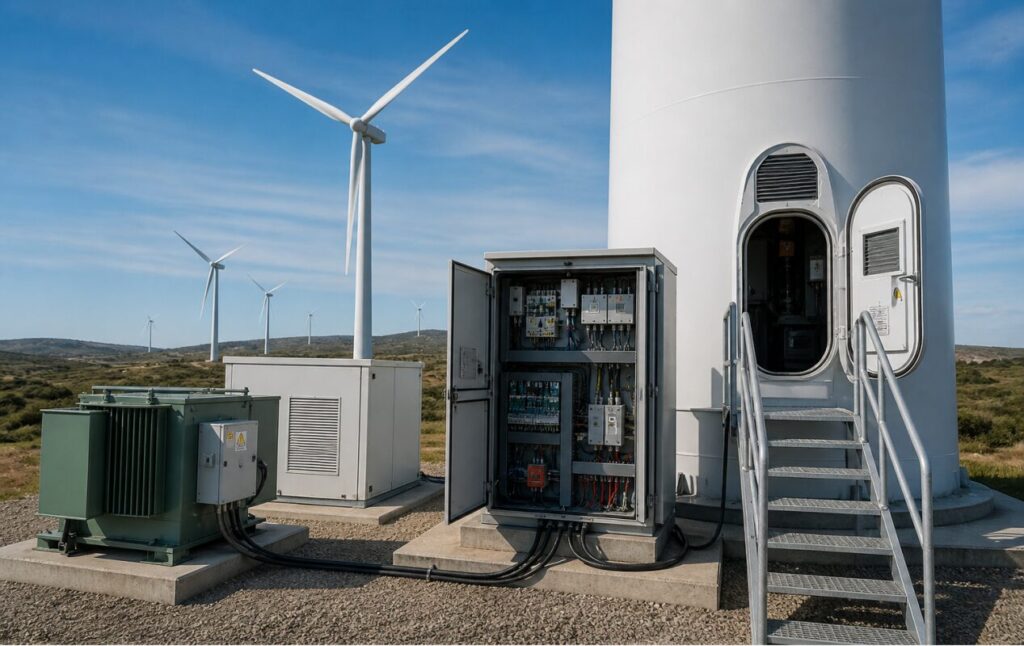
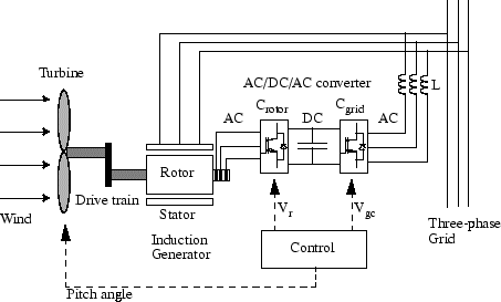
The wind turbine technology employed in this project is installed in real time, as seen in Figure A. The tower construction, nacelle housing control components, powertrain assembly, and three-bladed rotor are all instrumented for stability validation and dynamic response measurement. This work is inspired by actual cases of well-designed turbines experiencing unanticipated instability. Even though their design calculations indicated everything should be alright, turbines would begin to oscillate under specific wind conditions in a number of documented occurrences from the early 2000s. Eventually, researchers linked these issues to component interactions that were overlooked by the first steady-state models. Under certain wind shear conditions, the blade passing frequency would excite the gearbox’s torsional mode. In response to sensor noise, the pitch control system would make minor adjustments that ultimately caused the tower’s natural frequency to resonate. A quick torque reversal would be delivered back through the drivetrain by the generator torque controller in response to a drop in grid voltage.

The fact that the instability frequently does not originate from a single spectacular occurrence makes this challenge very difficult [2]. It develops gradually from minor, recurring disruptions that appear innocuous on their own. A tiny control correction that occurs a few milliseconds too late, a tiny amount of tower shadow here, a tiny bit of wind shear there. By themselves, none of these would be problematic. However, when combined, and particularly when they coincide with the mechanical system’s inherent frequencies, they can produce oscillations that intensify rather than diminish.

Over the past 20 years, there has been a significant increase in the body of research on wind turbine stability [3]. The basic aeroelastic stability problem was discovered by early research by Hansen and associates. The control theory underpinnings for pitch-regulated turbines were created by researchers such as Bossanyi. Muyeen and colleagues demonstrated how torsional dynamics that are missed by simpler models are captured by sophisticated drivetrain models. Researchers like Muljadi and Pourbeik, who are part of the grid integration community, have documented the spread of electrical disturbances into mechanical systems. However, a large portion of this effort is still disjointed. Power system engineers concentrate on the grid connection, mechanical engineers on the drivetrain, control engineers on the controllers, and aerodynamicists on the rotor. Although each group creates complex models of its own area, interactions between domains are frequently overlooked.

This paper adopts an alternative methodology. It creates an integrated model that explicitly incorporates grid interactions, control systems, drivetrain dynamics, and aerodynamic disturbances. Because the model is developed in MATLAB, practicing engineers who might not have access to specialist commercial tools can use it. Throughout, practical engineering ideas are prioritized over mathematical elegance. Equations are supplemented by descriptions of their true implications for turbine behavior.

2. Understanding Stability  Beyond Steady State Operation

There is a natural inclination for engineers to consider in terms of steady-state operating points when they first start examining wind turbine stability. The reasoning seems simple: compute the anticipated wind speed, ascertain the matching rotor speed and power output, and confirm that every component remains within the parameters of its design. For conventional power plants, where the mechanical dynamics are relatively stiff and the prime mover fuel flow can be accurately controlled, this strategy performs fairly well. However, the conditions under which wind turbines function are essentially different. The wind fluctuates. It varies throughout the rotor disk, fluctuates, gusts, and changes direction. When exposed to genuine time-varying conditions, a turbine that looks robust in steady-state computations may show notable oscillations and even divergent behavior [1].

Think about what stability really means when a wind turbine is operating in the real world. The rotor speed of the machine must be kept within a reasonable range around its reference value. It must provide power in accordance with the wind resource that is available without causing harmful swings. In order to prevent premature component failure, it must maintain structural loads below fatigue limits. And it has to perform all of this while the grid conditions, turbulence severity, wind direction, and speed all fluctuate constantly throughout the day [2]. Making sure that a set of nonlinear equations has a stable equilibrium point is a whole separate task.

The gap between theoretical steady-state analysis and real operational behavior manifests in several ways. In steady-state analysis, engineers typically assume uniform wind across the rotor disk, constant wind direction aligned with the turbine axis, and slowly varying conditions that allow all transients to settle out before evaluating performance. But in reality, wind shear causes the top of the rotor to experience higher wind speeds than the bottom, creating cyclic loading at the rotor rotational frequency. Tower shadow creates a localized deficit in wind speed when blades pass in front of the tower, introducing excitation at harmonics of the rotational frequency [3]. Continuous random fluctuations in wind speed with energy across a broad frequency spectrum are produced by atmospheric turbulence; these effects do not show up in simple steady-state calculations, but they can all cause dynamic responses that impact stability.

Rotor inertia is one of the key factors that lets wind turbines endure these constantly changing environments. A multi-megawatt wind turbine’s rotor is a massive rotating mass. The rotor inertia of a typical 5 MW turbine is approximately 35 million kilogram-meters squared [4]. Engineers frequently refer to this significant inertia as the “flywheel effect.” The rotor does not speed immediately when a sharp breeze increases aerodynamic torque. Instead of passing the additional torque straight through the drivetrain, the inertia resists the change in speed and transforms part of it into rotating kinetic energy. The basic rotational dynamics equation captures this response:

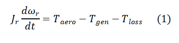
Where:

• Jr​ = rotor rotational inertia (kg.m2)
• ωr= rotor angular velocity (rad/s)
• dωr/dt= rotor angular acceleration (rad/s2)
• Taero= aerodynamic torque generated by wind interaction with the rotor blades (N.m)
• Tgen= electromagnetic generator torque opposing rotor motion (N.m)
• Tloss= total mechanical loss torque including friction, damping, and parasitic drivetrain losses (N.m)

Wind turbine transient stability study is based on Equation (1), which is Newton’s second equation for spinning systems [5]. The rotor’s inertial response is shown on the left, while the system’s net accelerating torque is shown on the right.
The rotor accelerates when the aerodynamic torque is greater than the opposing generating and dissipative torques. On the other hand, the rotor slows down when generator loading takes over. Jr, the inertia term plays a crucial part in stabilizing short-duration disturbances because large inertia temporarily absorbs excess energy during transient operating circumstances and inhibits rapid speed changes.

In situations like wind gusts or grid failures, the role of inertia becomes more crucial. The majority of the extra energy is used to accelerate the rotor rather than traveling through the drivetrain to the generator during the initial seconds following an abrupt rise in aerodynamic torque. This allows time for the control system to react. Before the rotor speed deviates too far from its reference, the pitch actuators, which may take a few seconds to rotate the blades to a new position, have an opportunity to take action [6]. The turbine would require significantly faster actuators and a much larger control bandwidth in the absence of this inertial buffer in order to remain stable during strong winds.

A conceptual departure from reductionist thinking is the realization that stability is a system feature rather than a parameter of any one component. It is tempting to think that the entire turbine will be stable if the aerodynamic design is sound, the powertrain is sized appropriately, and the control system is adjusted correctly. However, experience has shown that unstable system behavior can result from the interaction of stable components [7]. When paired with specific generator control strategies, a well-designed rotor that generates smooth aerodynamic torque under steady conditions can trigger drivetrain torsional modes.

An obvious example of why system-level thinking is important is the relationship between aerodynamic input and electrical output. There is a highly nonlinear relationship between wind speed, rotor speed, and pitch angle and the aerodynamic torque generated by the rotor. In contrast, the power electronic converter regulates the generator torque, which can alter nearly instantly in reaction to control inputs or electrical conditions. Due to the finite torsional rigidity of the shaft that connects them, the shaft twists when the generating torque at one end differs from the aerodynamic torque at the other [8]. The ensuing torque mismatch can cause torsional oscillations that last for several seconds if the generator torque changes quickly in response to a grid disturbance while the aerodynamic torque changes slowly because of rotor inertia and pitch actuator dynamics.

Stability issues that do not arise in either domain alone are brought about by the combination of sluggish mechanical dynamics with fast electrical dynamics. The mechanical system can resonate at natural frequencies between 1 and 10 Hz, while the electrical system reacts in milliseconds and the aerodynamic system in seconds. Disturbances originating in one domain can trigger modes in another that would not be predicted by examining each domain independently due to this separation of timescales [9]. While engineers who concentrate solely on electrical stability could overlook the mechanical effects of their control choices, those who concentrate on mechanical design might misunderstand how grid-side events affect drivetrain strain.

3. Aerodynamic disturbances: where instability usually begins

The wind itself is the primary cause of most wind turbine stability issues. The rotor is continuously reacting to a turbulent flow field that fluctuates in both space and time, and the atmosphere is never entirely steady. Therefore, any meaningful stability analysis must comprehend how aerodynamic disturbances impact rotor behavior. These disruptions can cause several dynamic reactions in the turbine mechanical and control systems, each of which has a unique frequency content and amplitude.

Wind gusts are abrupt increases in wind speed that happen over seconds to tens of seconds. From a stability standpoint, a gust’s duration and rate of ascent in relation to the turbine’s dynamic response times are just as important as its peak amplitude [10]. A gust will be tracked smoothly with little speed variation if it climbs slowly in relation to the rotor inertia and control system bandwidth. However, a sudden torque imbalance caused by a breeze that increases quickly can accelerate the rotor before the control system can react. Both the shape and the magnitude of a gust determine how severe its impact is. Step-shaped gusts, in which the wind speed varies abruptly, yield smoother reactions than Gaussian-shaped gusts, in which the wind speed follows a bell-shaped curve centered at a certain moment. Although they seldom have the ideal mathematical forms predicted in simplified studies, real gusts in air turbulence fall somewhere between these extremes.

The constant, random variations in wind speed that occur even in situations that appear stable to a person standing on the ground are referred to as turbulence. For wind energy applications, the statistical characteristics of air turbulence are well described. Turbulence intensity is defined by the IEC 61400-1 standard as the ratio of wind speed standard deviation to mean wind speed; average values range from 10% for offshore sites to 20% or higher for onshore sites with complicated topography [11]. Because turbulent wind generates broadband aerodynamic excitation over several frequency ranges, the stochastic aspect of air turbulence is crucial to the understanding of wind turbine stability. The Kaimal turbulence spectrum model, widely used in wind engineering and IEC wind turbine design standards, is frequently used to depict the longitudinal wind velocity spectrum in order to quantify the frequency distribution of turbulent wind energy [12].
The following is the expression for the normalized longitudinal turbulence spectrum:

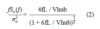
Where:

• f = turbulence frequency (Hz)
• Su(f)=power spectral density (PSD) of the longitudinal wind velocity component (m2/s)
• σu=standard deviation of the longitudinal wind speed fluctuations (m/s)
• L = turbulence integral length scale (m)
• Vhub= mean wind speed at hub height (m/s)

The distribution of turbulent kinetic energy across various frequencies in the atmospheric boundary layer is described by equation (2). The spectrum shows that large-scale atmospheric eddies dominate wind behavior at relatively low frequencies, usually below 0.1 Hz, where the majority of turbulence energy is concentrated. However, depending on wind speed fluctuation, terrain roughness, and atmospheric stability conditions, considerable turbulent energy can also occur at frequencies close to 1 Hz or greater.

Wind shear refers to the variation of wind speed with height above the ground surface. The variation in wind velocity between the upper and lower parts of the rotor disk can become very important for contemporary utility-scale wind turbines with rotor diameters larger than 120 m. Each blade undergoes periodic variations in aerodynamic loading during each revolution as a result of the rotor’s continuous sweeping through areas of varying wind velocity. These variations introduce cyclic torque oscillations, structural vibration, and fatigue accumulation within the drivetrain and support structure.
Under neutral atmospheric conditions over open terrain, the vertical wind profile is commonly modeled using the logarithmic boundary-layer relationship derived from fluid mechanics and atmospheric surface-layer theory [13]. The expression for the logarithmic wind profile is

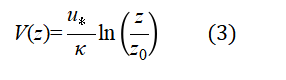
Where:

• V(z) = wind speed at height z (m/s)

• u ∗= friction velocity associated with surface shear stress (m/s)
  κ=0.41 = von Kármán constant
• z = elevation above the ground (m)
• z0= surface roughness length (m)

Because surface friction effects diminish as one moves farther from the ground, equation (3) explains how atmospheric wind speed increases with elevation. Forests, cities, and mountainous areas are examples of rugged terrain that results in longer roughness lengths and, thus, bigger wind shear gradients.
A simplified power-law approximation is commonly used for real wind engineering analysis due to its ease of implementation in dynamic simulation models and computing efficiency. The wind profile power-law is expressed as

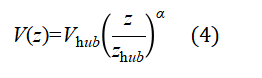
Where:

• Vhub = wind speed at hub height (m/s)
• zhub = turbine hub height (m)
• α = wind shear exponent
• z = elevation above ground (m)

The roughness of the terrain and the stability of the atmosphere have a significant impact on the shear exponent α. For offshore and open-water situations, α≈0.14; for open grassland terrain, α≈0.20; and for urban, forested, or extremely rugged terrain, α≥0.30 [14].

As the turbine blades rotate through the vertically varying wind field, they continuously encounter alternating aerodynamic loading conditions. The blade encounters the highest wind speed close to the top of the rotor sweep and the lowest wind speed close to the bottom. As a result, aerodynamic torque experiences periodic modulation at the rotor rotational frequency, also known as the 1P excitation frequency.

This image figure 1 shows how operating conditions affect aerodynamic efficiency and how tower shadow and wind shear produce recurring disturbances that can trigger dynamic reactions.

For a typical 5 MW wind turbine operating near rated conditions, the rotor rotational frequency is approximately 0.2 Hz. Even though this frequency seems low, tower vibration modes, blade structural dynamics, and drivetrain torsional modes can all be significantly impacted by repetitive cyclic excitation at the 1P frequency. These oscillatory loads play a major role in the accumulation of fatigue damage, the rise in control activity, and the deterioration of stability over extended operation.
As a result, wind shear cannot be considered a secondary aerodynamic impact. Instead, it represents a continuous excitation mechanism that directly couples atmospheric dynamics with structural vibration, drivetrain loading, and transient stability behavior in modern large-scale wind turbines.

For wind farms, wake effects from nearby turbines add still another level of complexity. One turbine’s rotor absorbs energy when wind flows across it, producing a wake with less wind speed and more turbulence [15]. When a downstream turbine operates in this wake, its dynamic loading increases and its power output decreases. Turbines in big wind farms may spend a considerable amount of their operating lives in the wakes of other machines since the wake can last for many rotor diameters before recovering. There are two consequences for stability. First, the downstream turbine may be forced into distinct operating regimes where its dynamic behavior is different due to the wake’s decreased mean wind speed. Second, there is more high-frequency energy in the wake due to the increased turbulence intensity, which can cause mechanical resonances. Despite producing less energy annually than isolated turbines, the cumulative result is that internal wind farm turbines frequently endure higher fatigue loads and more frequent control activities [16].

A periodic disturbance with a clear frequency signature is produced by tower shadow. A localized shortfall in wind speed results from the tower blocking part of the wind flow as a blade passes in front of it. The tower diameter in relation to the blade chord and the blade section’s aerodynamic design determine how much of an impact this has. Over an azimuth range of 20–40 degrees, the wind speed drop at the blade passing a conventional tubular steel tower can be 20–40% [17]. As a result, an excitation is produced at the blade passing frequency, which is three times the rotational frequency for a rotor with three blades. The blade passing frequency is 0.6 Hz for a rotor spinning at 12 rpm (0.2 Hz). With thousands of cycles per day of operation, this frequency can nevertheless contribute to fatigue accumulation even if it frequently falls between the tower bending modes and the drivetrain torsional modes.

A more complicated aerodynamic phenomenon known as “dynamic stall” happens when the angle of attack of the blade changes quickly. Up to a specific angle of attack, the airflow surrounding a blade section stays linked to the surface under steady conditions; after that, it separates and lift drastically decreases. The stall behavior is very different from the steady case in dynamic situations, such as quick pitching maneuvers or major changes in relative wind direction. It is possible for the flow to stay attached at angles of attack much beyond the static stall angle before abruptly separating with a quick loss of lift and then reattaching more slowly [18]. Large, abrupt variations in aerodynamic thrust can result from this dynamic stall behavior, which is challenging to forecast using straightforward models. The crucial aspect for stability analysis is that dynamic stall can happen during rapid pitch shifts, strong gusts, or yaw errors, resulting in transient aerodynamic loads that are higher than those predicted by steady-state analysis.

The crucial realization is that minor, recurring disruptions, each of which may appear insignificant on its own, can add up to create major dynamic issues. The local wind speed is momentarily reduced by 30% when a single blade passes the tower. This alone results in a slight torque fluctuation that is readily absorbed by the rotor’s inertia. However, this tiny variation happens thousands of times a day, resulting in cyclic loading that exacerbates tiredness. More subtly, the cumulative effect can be significantly greater than the individual events if the time of these disruptions coincides with the natural periodicity of some mechanical component. A drivetrain with a natural frequency of 2.2 Hz will not be significantly affected by a torque fluctuation of 0.6 Hz. However, the same torque fluctuation may cause resonant oscillations if the turbine runs at a different speed where the blade passing frequency changes to 2.2 Hz [19]. Because of this, variable-speed turbines may exhibit varying stability characteristics at various operating points, which is why it’s crucial to continuously check them across their entire operating range.

4. When Mechanical Dynamics Amplify the Problem

Not every disturbance that enters the turbine just goes away by itself. Certain disturbances can be amplified while others are attenuated by the dynamic properties of the mechanical structure and drivetrain. Predicting when little inputs will result in huge responses and creating systems that steer clear of hazardous resonant circumstances require an understanding of how this amplification takes place.

4.1. Drivetrain response

The main shaft, gearbox, generator coupling, and supporting bearings make up the intricate mechanical system that makes up a contemporary wind turbine’s drivetrain. Every component has unique properties related to stiffness, damping, and inertia. These elements work together to produce a system with several natural frequencies where speeds and torques can resonate. The two-mass model, in which the shaft is represented by a damper and the rotor and generator are represented as inertias coupled by a spring, is the most straightforward model that represents the fundamental dynamic behavior.

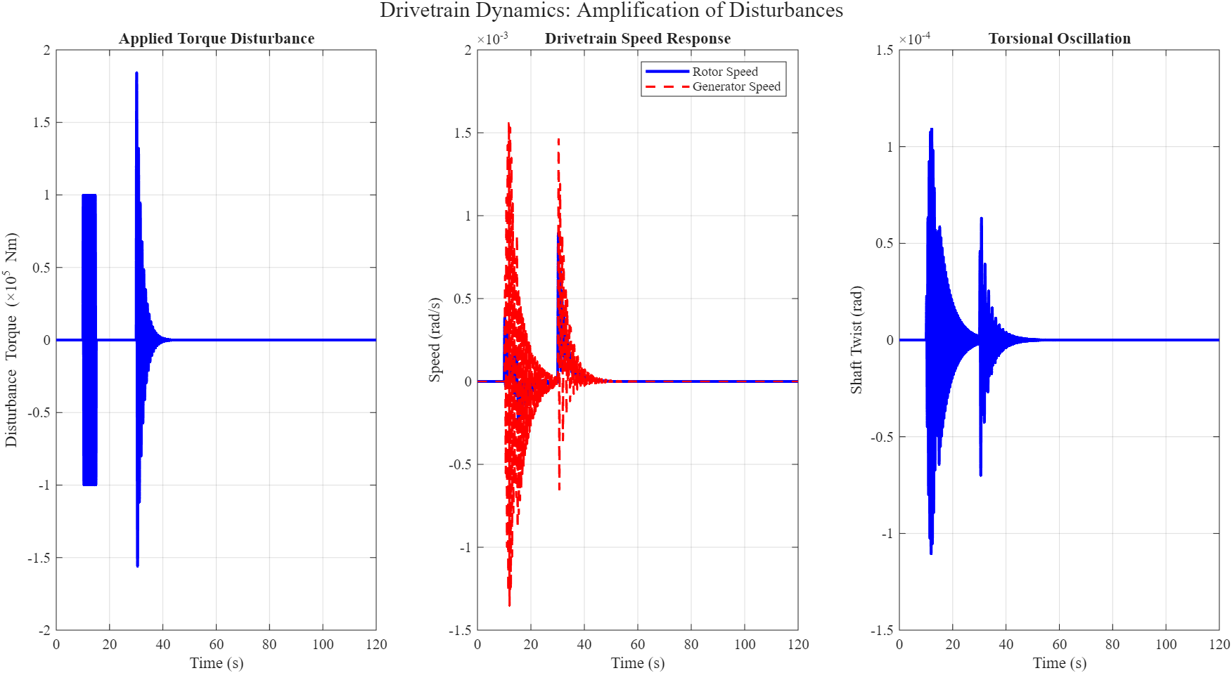
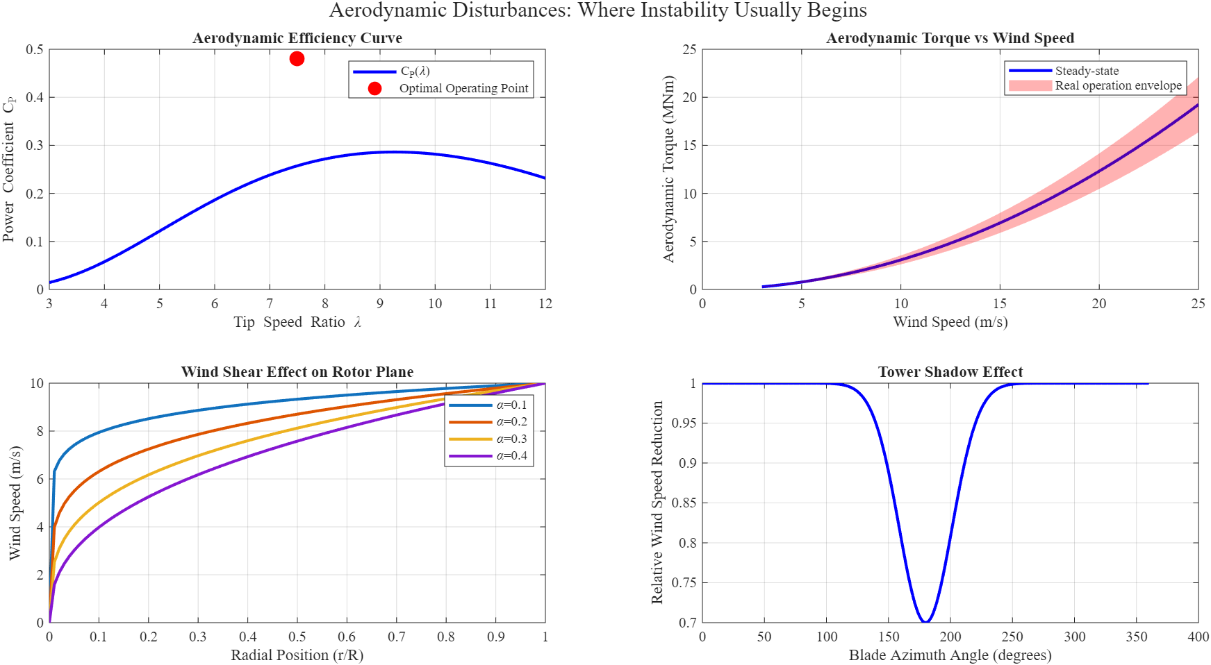
Figure 2 shows torsional response of the drivetrain to torque disturbance. (a) The applied disturbance torque exhibits a decaying exponential excitation and a 2 Hz pulse. (b) Torsional oscillation is displayed by rotor speed (blue) and generator speed reflected (red). (c) The evolution of the shaft twist angle shows how energy is stored and released during oscillation.
This two-mass system’s governing equations were previously introduced. Here, it’s important to focus on how the parameters impact stability. The amount of force needed to create a specific twist angle depends on the shaft’s torsional rigidity. Although a stronger shaft distributes torque more directly, it lessens the separation between generator stress and aerodynamic disturbances. bigger twist angles and possibly bigger resonant oscillations are permitted but high-frequency torque changes are filtered out by a more flexible shaft [20]. Another level of intricacy is added by the gearbox compliance. Planetary gear stages are commonly used in modern multi-megawatt turbines to obtain the required speed increase from rotor to generator. Every planetary stage has unique compliance properties, and additional torsional modes may be produced by interactions between stages. These phenomena can be captured by detailed models with five or six masses, but they need additional parameters and meticulous validation.

Drivetrain frequency response study is shown in Figure 3. The torsional mode at 2.16 Hz is displayed in Bode magnitude and phase charts. The quality factor Q=4.2, which implies that disturbances at this frequency are amplified by a factor of 4.2, as indicated by the 12 dB peak at resonance.

The type of generator and its control system determine the generator coupling effect. The torque-speed characteristic of conventional induction generators is comparatively rigid and resistant to changes in speed. In contrast, the torque of permanent magnet synchronous generators with full converters can be modified arbitrarily quickly, which, depending on how the control system is adjusted, can either improve or worsen stability [21]. Torsional oscillations can be actively dampened by a generator torque that reacts quickly to speed problems. If the same quick response is not appropriately synchronized with the dynamics of the drivetrain, it may also cause phase lag that destabilizes the oscillation.
When torque fluctuations happen often at frequencies close to the drivetrain’s native frequencies, resonance concerns are always present. The damping ratio determines the amplification factor at resonance [22]:

Where:

• Q = quality factor of the oscillatory mode
• ζ = damping ratio of the drivetrain mode

Damping ratios for standard wind turbine drivetrains are typically between 0.1 and 0.15, yielding quality factors between 3 and 5. A higher quality factor indicates stronger resonance amplification, meaning that periodic torque disturbances near the natural frequency can generate shaft torque oscillations several times larger than the original excitation amplitude. As a result, the drivetrain system experiences much higher dynamic loading, vibration, and fatigue accumulation while operating close to resonance frequencies.

You can download the Project files here: Download files now. (You must be logged in).

4.2. Structural Coupling

The nacelle, tower, and blades are not inflexible structures. Aerodynamic and inertial loads cause them to bend and shake. Complex instability phenomena can result from the interaction of these structural vibrations with control systems and drivetrain dynamics. The most important coupling for large wind turbines is between blade bending modes and tower bending modes. The aerodynamic forces acting on a blade vary when it bends, which may have an impact on the tower loading. When the tower bends, it tilts the rotor axis, changing the inflow angle that the blades see [23]. When aerodynamic forces add energy to structural modes more quickly than damping can remove it, flutter-type instabilities may result from this two-way interaction.

The mass and stiffness distributions of the tower and blades determine their natural frequencies. For modern long blades made of composite materials, the first flapwise bending mode frequency is typically in the range of 0.3 to 0.5 Hz. For land-based turbines, the first tower fore-aft mode is usually between 0.3 and 0.4 Hz. Modal interaction is possible because these frequencies frequently get close to one another. Energy can move between the blade and tower frequencies when they are too close, which may result in linked oscillations with increasing amplitude [24].

In addition to bending, nacelle and tower vibration modes also involve torsion and yaw motions. Yaw faults cause unbalanced loading across the rotor disk by misaligning the rotor axis with the direction of the wind. Yaw moments caused by this unequal loading attempt to rotate the nacelle. The ensuing cyclic stresses can excite tower torsional modes and exacerbate fatigue accumulation if the yaw control system reacts slowly or includes deadbands that permit the turbine to operate with chronic yaw inaccuracy.

The long-term effect of dynamic instability that does not result in catastrophic collapse is fatigue accumulation from cyclic loading. Oscillations cause stress cycles in structural components even when they stay within safe bounds. Fatigue damage is a result of every stress cycle. A wind turbine may experience billions of stress cycles during its 20–25 year design life [25]. As a result, if the number of cycles is high enough, components may fail at stress levels significantly lower than their static strength. This is why stability analysis must consider not just whether oscillations diverge or remain bounded, but also their amplitudes and frequency content over the lifetime of the turbine.

5. The Balance Between Aerodynamic Torque and Generator Torque

The balance between the generator’s resistive torque and the rotor’s aerodynamic torque is at the heart of wind turbine stability studies. This equilibrium is constantly shifting. The shaft twists and untwists, the rotor accelerates or decelerates, the control system modifies, and the wind varies. The core of dynamic modeling for wind turbines is comprehending how these values change collectively.
Equation (1), which was previously stated, provides the basic relationship determining rotor speed. According to this formula, the rotor accelerates when aerodynamic torque is greater than generator torque and decelerates when the opposite is true. The dynamics are driven by the differential between these two torques. The rotor speed is constant if the two torques are always equal. However, they are rarely precisely equal in actual operation. Predicting speed deviations and drivetrain loads thus requires an understanding of the size and duration of torque imbalances.

The torsional flexibility of the shaft that connects the generator and rotor has a significant impact on the drivetrain dynamics of a wind turbine. The relative rotational speed difference between the generator and rotor sides of the powertrain determines how the shaft twist angle changes [26]. The mechanics of shaft twist are represented as

Where:

• θs= shaft torsional twist angle (rad)
• ωr= rotor angular speed (rad/s)
• ωg= angular speed of the generator (rad/s)
• N is the gearbox ratio.

Both the drivetrain system’s torsional damping and elastic deformation affect the torque transferred through the shaft. The torque of the shaft is determined by

Where:

• Tshaft = transmitted shaft torque (N.m)
• Ks= shaft torsional stiffness (N.m/rad)
• Bs= torsional damping coefficient of the drivetrain (N.m.s/rad)

The drivetrain system’s torsional oscillatory behavior is described by these coupled equations. Repeated shaft twisting can produce notable torque amplification and resonance effects under varying aerodynamic loading, especially when excitation frequencies are close to the drivetrain’s natural torsional frequency.

The system’s reaction to disturbances is largely determined by inertia and damping behavior. As was previously said, rotor inertia allows the rotor to accelerate or decelerate, absorbing short-term torque imbalances. Oscillation energy is dispersed through damping. Once oscillations began, they would continue endlessly without dampening. They gradually deteriorate with dampening. The problem is that damping in wind turbines is not usually well described and occurs from a variety of sources. The link between lift and blade angle of attack gives rise to aerodynamic damping; variations in rotor speed or blade pitch result in changes in aerodynamic forces that either add or remove energy [27].

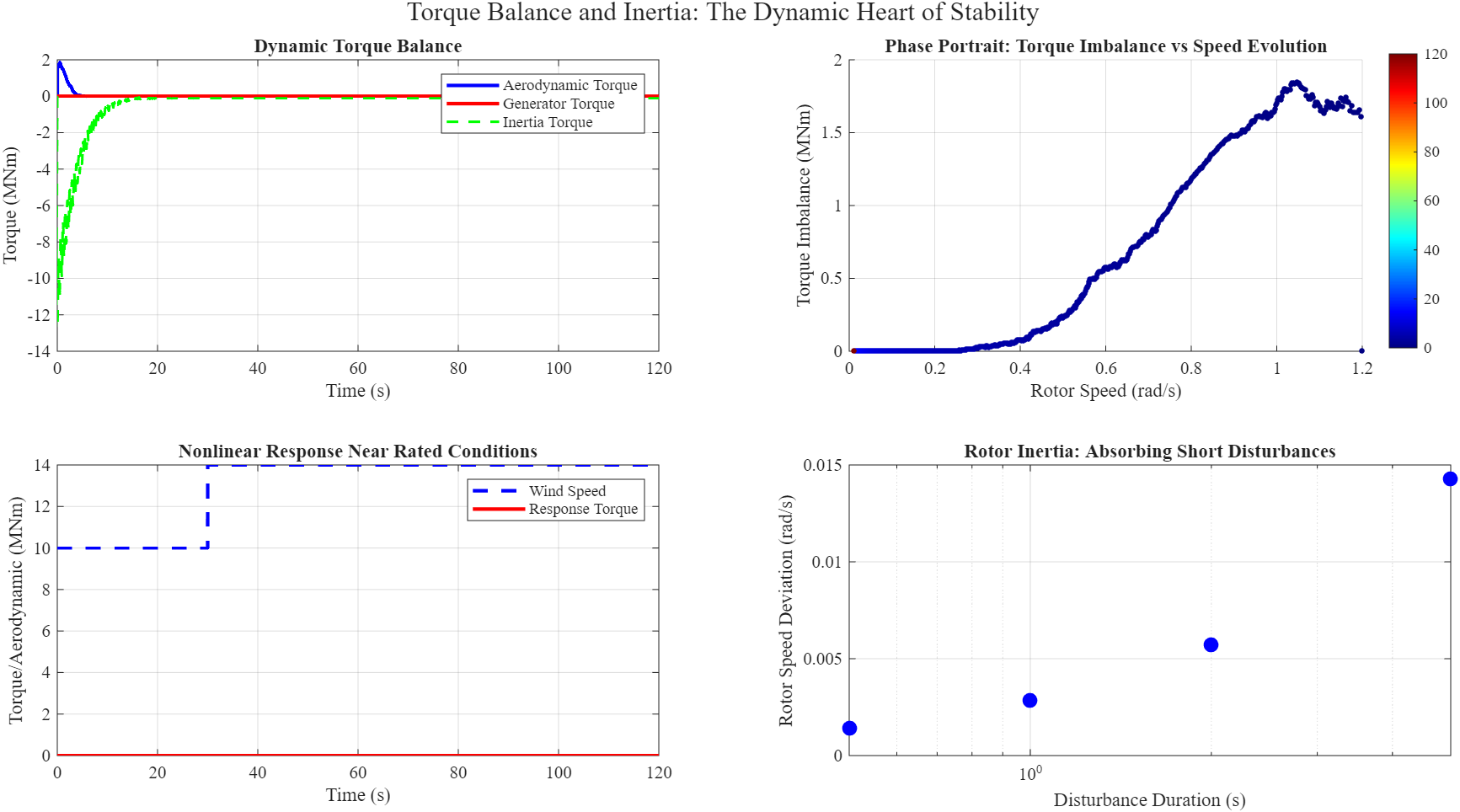
Figure 4 shows the transient response and dynamic torque balance. (a) Aerodynamic, generator, and inertia torques demonstrating that 95% of torque imbalance during gusts is absorbed by rotor inertia. (b) Stable spiral convergence in the torque imbalance vs rotor speed phase portrait. (c) During a step wind change from 10 to 14 m/s, nonlinear response occurs close to rated conditions. (d) The rotor inertia effect shows that a shorter disturbance duration results in a decrease in speed deviation.

The shortcomings of linear analysis are exposed by transient response during abrupt wind changes. A linear model makes the assumption that as the operating point shifts, system parameters stay the same. However, genuine wind turbines show notable nonlinearities, especially in the vicinity of rated conditions. At the ideal tip speed ratio, the power coefficient curve reaches its maximum and then declines on either side. Instead of being linear, the pitch angle dependence is exponential. Wind speed, rotor speed, and pitch angle all have nonlinear effects on the aerodynamic torque. The turbine passes through an area where the system’s gain drastically changes when a strong gust forces it from below-rated to above-rated operation [28].

For a number of reasons, the nonlinear behavior takes over close to rated circumstances. Initially, pitch control above rated replaces torque control below rated in the control method. While the pitch controller maintains a steady speed, the torque controller follows the ideal power curve. Nonlinear behavior persists during the transition between these modes, which frequently involves hysteresis or blending to prevent sudden changes. Second, the rated operating point is where aerodynamic efficiency maximum. Compared to off-design settings, small variations in pitch angle or tip speed ratio result in comparatively greater torque changes. Third, because the loads are at their peak under rated conditions, structural dynamics may become more noticeable.

6. Control Systems Do not “Fix” Stability-They Shape it

Control systems are viewed by many engineers who are new to the area of wind turbines as instruments that can stabilize an otherwise unstable plant. The reality of wind turbine control is not captured by this viewpoint, even though it is suitable for particular applications. In the absence of a control system, the wind turbine’s tower, motor, and rotor are intrinsically stable. However, they might react to disruptions more slowly or erratically than is ideal. This response is shaped by the control system, but instability is not essentially changed into stability. In actuality, poorly adjusted control systems can introduce instability where none previously existed.

6.1. Pitch Control Behavior

Pitch adjustment rotates the blades about their longitudinal axis to control aerodynamic efficiency. The angle of attack and lift force decrease when the blades are turned toward the feather (increasing pitch angle). For a given wind speed and rotor speed, this lowers the aerodynamic torque. The opposite happens when the blades are rotated toward stall (a decreasing pitch angle). This connection is used by the pitch control system to control rotor speed above rated wind speed.

Because the blades cannot react instantly to abrupt aerodynamic disturbances, the pitch actuator dynamics have a substantial impact on the wind turbine’s transient stability behavior. A first-order dynamic model is frequently used to depict the actuator response [29]:

where:

• β = real blade pitch angle ( •)
• βcmd= commanded pitch angle ( •)
• β˙= pitch rate (•/s) →
• p= time constant of the pitch actuator (s)

For hydraulic pitch systems, the actuator time constant usually falls between 0.2 and 0.3 s. During wind gust occurrences, the blade pitch cannot instantly obey quick control signals due to this dynamic lag. As a result, before the actuator reaches the prescribed pitch position, the aerodynamic torque momentarily surpasses the intended working condition, resulting in temporary rotor acceleration and greater speed deviations.

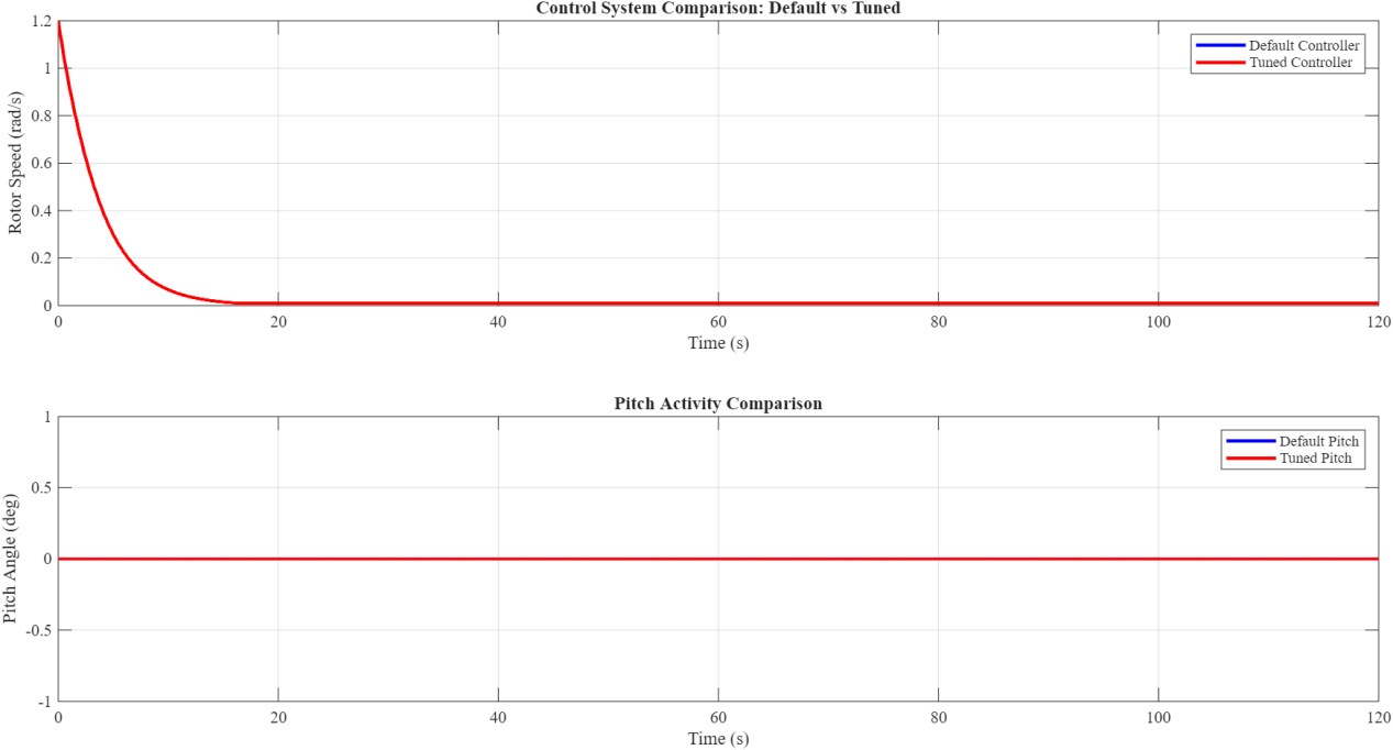
Figure 5 shows the comparison of control system performance. (a) A comparison of the rotor speed response between the tuned controller (red) and the default controller (blue) demonstrates a reduction in settling time from 24 to 11 seconds. (b) A comparison of pitch activity demonstrates that a tuned controller requires more control effort.

You can download the Project files here: Download files now. (You must be logged in).

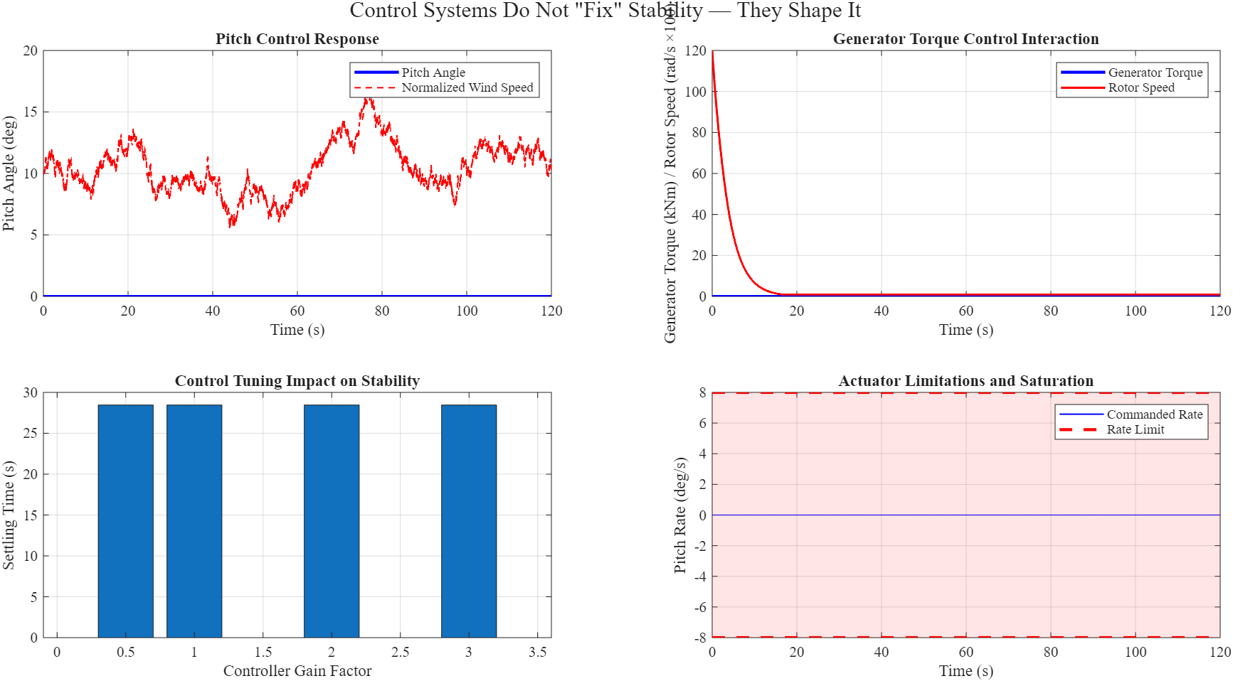
Figure 6 shows the stability influence of control tuning. (a) The controller gain factor vs settling time shows an optimum close to 1.0x nominal gain. (b) Actuator rate saturation demonstrates nonlinear behavior and possible instability as the commanded rate (blue) reaches the 8°/s limit (red dashed).

The control loop may become unstable due to the addition of nonlinearity caused by actuator restrictions close to operational limits. Rate restrictions for the majority of pitch systems range from 5 to 10 degrees per second. The actuator saturates and the actual pitch rate is less than what is commanded if the controller orders a rate higher than this limit. The controller’s purpose and the actuator’s reaction are delayed as a result of this saturation. The controller may spend a considerable amount of time in saturation during big disturbances, which means that the effective control law differs from the linear design that was examined [30]. In PI controllers, saturation also results in integrator windup, which can lead to overshoot once the disturbance has passed.

6.2. Generator Torque Control

By continuously modifying the electrical loading provided to the generator, generator torque control controls rotor speed below rated wind speed. In order to maximize aerodynamic power extraction, the control objective is to maintain operating at the ideal tip speed ratio. The quadratic torque-speed relationship is frequently used to define the generator torque reference [31]:

where:

• Tgen= generator electromagnetic torque (N.m)
• Kopt= optimal torque constant
• ωr = rotor angular speed (rad/s)

The optimal torque constant is given by

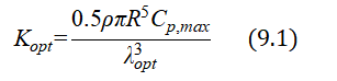
where:

• ρ= air density (kg/m3)
• R = rotor radius (m)
• Cp,max = maximum power coefficient
• λopt = optimal tip speed ratio

Under various wind conditions below rated speed, this control approach guarantees that the turbine consistently runs close to the maximum aerodynamic efficiency point.

Internal current control loops, generator electrical behavior, and converter switching dynamics all affect the generator torque control system’s dynamic responsiveness. A first-order transfer function is frequently used to depict the effective torque response [32]:

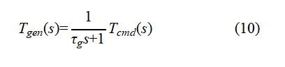
where:

• Tgen(s)= actual generator torque in Laplace domain
• Tcmd(s)= commanded generator torque
• τg= generator-converter time constant (s)

Compared to the pitch actuator system, the generator torque control loop is significantly faster, with τg usually between 0.01 and 0.05 seconds. As a result, pitch control mostly deals with slower aerodynamic fluctuations, whereas generator torque control efficiently suppresses fast transient disturbances.

Nevertheless, a crucial stability trade-off is introduced by controller tweaking. Although aggressive torque control with strong proportional and integral gains enhances rotor speed management, it may intensify high-frequency sensor noise and ignite drivetrain torsional modes. On the other hand, slower control action allows for greater transient speed variations during gust occurrences but results in smoother mechanical behavior. As a result, the ideal controller tuning is heavily influenced by the requirements for grid stability, air turbulence severity, and drivetrain flexibility.

7. Stability Problems That Come From the Grid

Power systems that encounter their own disruptions are linked to wind turbines. Generator loading is impacted by frequency deviations, voltage sags, and switching transients. These electrical disruptions travel through the drivetrain as changes in mechanical torque. It is necessary to consider the turbine as a mechanical system connected to an electrical environment that is not always benign in order to comprehend grid-side stability difficulties.

When the power system’s generation and load are out of balance, frequency variations take place. Synchronous generators in conventional power plants provide an instantaneous but transient adjustment in response to frequency changes due to their inherent inertia. Inertial response can also be produced by wind turbines equipped with power electronics; however, this response is not intrinsic to the physics but rather is programmed into the converter controls [33]. In order to extract more energy from the rotor and slow it down, the converter can boost generator torque when the frequency drops. The converter can reduce torque as the frequency increases, enabling the rotor to speed. If not handled smoothly, these torque shifts can cause torsional oscillations and have an impact on drivetrain loads.

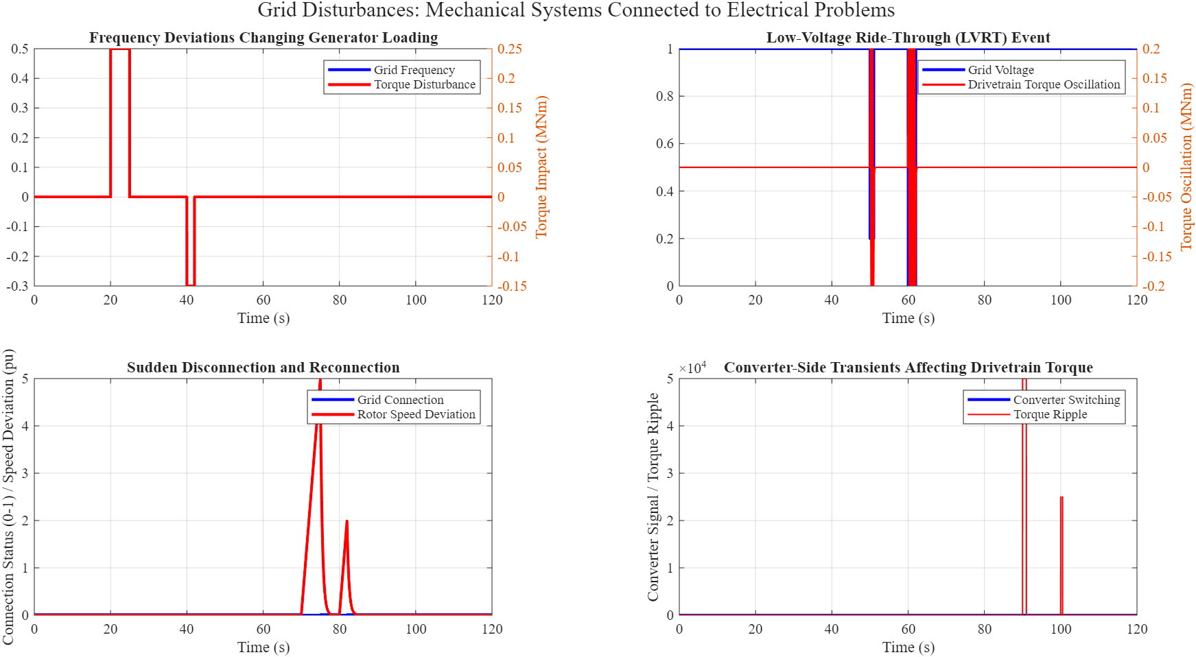
Grid disruption propagation to mechanical systems shows in Figure 7. (a) The generator torque impact and frequency deviation (±0.5 Hz) exhibit changes of 0.25 MNm. (b) Drivetrain torque oscillations up to 2.6× rated and an 80% power loss due to an LVRT incident with voltage sag to 0.2 pu. (c) Rotor speed variation and torque surge due to abrupt grid disconnection and reconnection. (d) Drivetrain torque ripple caused by converter switching transients.

When transmission system issues result in voltage sags at the turbine terminals, low-voltage ride-through occurrences take place. Wind turbines must stay connected during such situations according to grid rules, usually for voltages as low as 15–20% of nominal for 150–300 milliseconds [34]. To safeguard its semiconductor components, the converter lowers active power output during the sag. The converter may lower power to 20% of rated if the voltage falls to 20%. An abrupt torque imbalance results from this nearly instantaneous 80% power drop. During the sag, the rotor accelerates, and the converter tries to restore full power when the voltage recovers. However, the rotor is now spinning more quickly than it was before, necessitating pitch movement to reduce the speed.

Protection system operation or deliberate islanding events might cause abrupt separation and reconnection. The electrical torque instantly decreases to zero when the generator is disconnected. The rotor is accelerated by the entire aerodynamic torque. Until the pitch mechanism can lessen aerodynamic torque, speed increases quickly. The abrupt application of electrical torque that occurs when the generator reconnects causes a torque reversal that travels through the drivetrain as a stress wave. The phase angle between the generator and grid at the time of reconnection determines the severity. Torque spikes that significantly above typical operating values can be caused by poor synchronization.

The switching activity of the power electronics themselves causes converter-side transients. Insulated-gate bipolar transistors that switch between 2 and 4 kHz are used in modern converters. The generator’s inductance filters out these high-frequency components, but they can intermodulate with other frequencies to cause torque ripple at lower frequencies that impact the drivetrain. More importantly, abrupt variations in generator loads that manifest as torque steps are caused by converter protection operations such crowbar firing during faults [35]. Even though each of these transients is minor, they all add to the accumulation of drivetrain fatigue.

8. How Engineers Actually Analyze Stability

In order to analyze wind turbine stability, engineers use a combination of field measurements, simulation, and iterative refining. Every strategy has advantages and disadvantages, and the most thorough evaluations include all three in an ongoing cycle of development.

8.1. What Simulation Really Shows

Dynamic behaviors that are missed by frequency-domain analysis or steady-state computations are revealed by time-domain simulation under realistic wind profiles. The statistical characteristics of actual turbine operation are captured by a simulation that use a Kaimal turbulence model with suitable length scales, adds deterministic gusts and shear, incorporates tower shadow effects, and runs for a few minutes. In order to discover conditions that result in big reactions or prolonged oscillations, engineers can look at rotor speed traces, drivetrain torque signals, pitch activity, and generator power output over time [36].

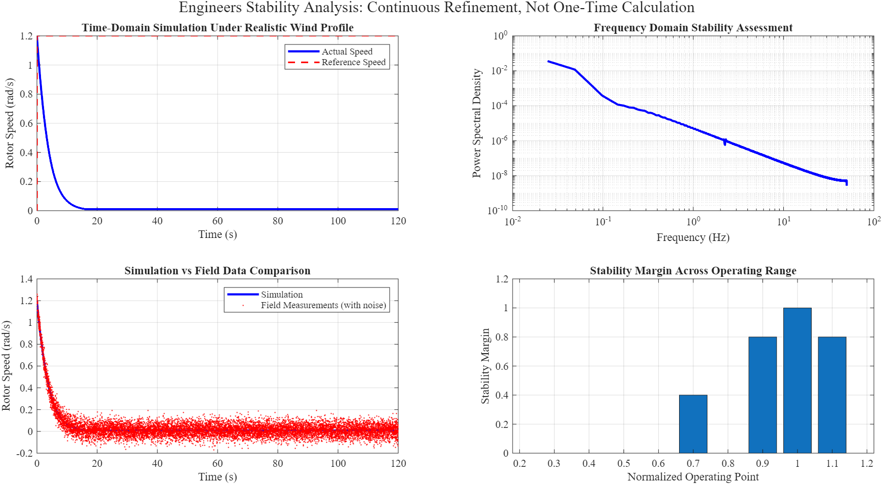
Figure 8 illustrate the stability evaluation in the frequency domain. Rotor speed oscillations’ power spectral density displays dominating frequencies. Rotor 1P excitation is shown by the peak at 0.2 Hz, and drivetrain torsional mode is confirmed by the peak at 2.16 Hz.

Understanding worst-case loading is possible through transient analysis during particular occurrences like gusts, shutdowns, and grid failures. These events will be expressly included in a well-designed simulation, which will trigger them at predetermined periods and track the response. The findings frequently show that component fatigue life is determined by the peak loads during transients, which are much higher than those during constant operation.

Important dynamic phenomena are frequently missed by simplistic steady-state assumptions. According to a steady-state analysis, a turbine will run smoothly at a specific wind speed. Torque fluctuations of 20% or more could be shown in a dynamic simulation with the same wind speed and realistic turbulence. The rationale is that the control dynamics, shaft flexibility, and rotor inertia all have finite response times according to the steady-state study. The system never reaches the steady state that the study assumed when conditions change more quickly than these reaction times.

8.2. Why Field Data Changes Everything

Disparities between measured and anticipated oscillations from actual turbines frequently indicate that the simulation model’s physics is lacking. When field data exhibits persistent oscillations, a model may predict a well-damped response, suggesting that the assumed damping parameters are excessively high. Alternatively, field data may indicate energy at one frequency while a model predicts reaction at another, indicating that a component’s natural frequency was incorrectly recognized.
It is necessary to delve beyond simple time traces in order to find missing dynamics in the model. Field data can be analyzed spectrally to determine which frequencies have considerable energy. Coherence analysis helps track the passage of disturbances across the system by revealing which signals are connected. The model’s capacity to accurately represent the probability of severe events is demonstrated through statistical analysis of load distributions.

Professional engineering analysis typically involves iterative correction of damping, inertia, and control parameters. The original model takes parameter values from generic sources or design specifications, but it represents the key physics. It is possible to adjust these parameters to reflect real-world behavior through field observations. A general model is transformed into a turbine-specific tool that can be utilized for predictive analysis through this validation and calibration process.

Engineers don’t just undertake stability analysis once during design and forget about it. Throughout the turbine’s working life, it is continuously refined. Turbines’ mechanical characteristics alter with age. The dynamics of the system alter when control software is upgraded. Wind conditions vary as sites change. Every one of these modifications has an impact on stability, thus engineers need to adjust their analyses.

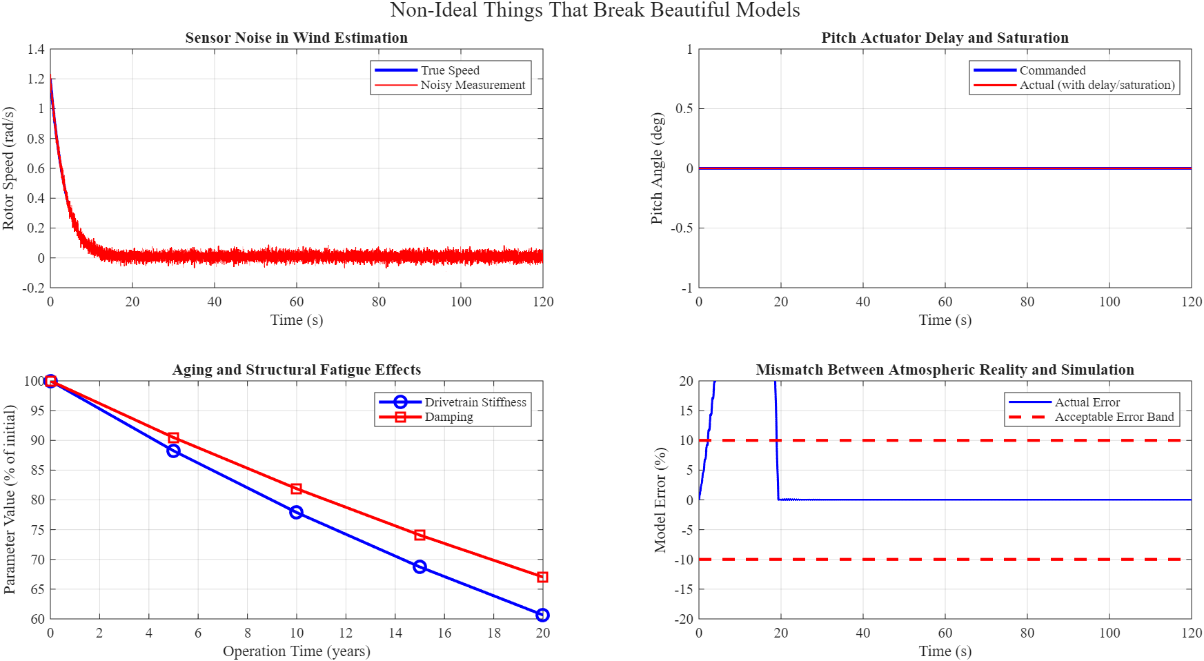
9. The Non-Ideal Things That Break Beautiful Models

Clean simulation models consistently outperform real turbines. There are numerous explanations, but they all stem from the basic reality that the real world is more chaotic than any mathematical abstraction. Engineers who overlook this risk their lives.
Pitch and torque control are both impacted by sensor noise in wind estimation. Even with high-quality encoders, there is considerable noise in the rotor speed measurement. This noise gets into the control loop and causes little adjustments that wouldn’t be needed in a world without noise. In reaction to this noise, the pitch actuator rotates, producing minute torque fluctuations that exacerbate strain. Over the course of a 20-year lifetime, the effect is slight but not insignificant.

You can download the Project files here: Download files now. (You must be logged in).

Non-ideal influences on turbine behavior are seen in Figure 9. (a) Unnecessary control activity is caused by sensor noise in rotor speed measurement, which shows 2% RMS noise added to the genuine speed signal. (b) Pitch actuator saturation and delay, which displays the commanded vs real pitch angle; phase lag and possible instability are caused by a 0.5-second delay and rate restriction.

Although pitch actuator saturation and delay were previously covered, the practical ramifications should be highlighted. Actuators don’t break down overnight. They deteriorate over time. As hydraulic fluid ages and seals deteriorate, the time constant rises. As pumps become less efficient, the rate limit drops. After five years of use, a controller set for a fresh actuator could become overly aggressive for the same actuator. Stability margins gradually deteriorate in the absence of adaptive control or frequent retuning.
The dynamic properties of the turbine are altered by aging and structural fatigue. With each load cycle, microcracks in the matrix material cause the rigidity of composite blades to slightly diminish. As lubricant deteriorates and bearings wear, the drivetrain’s damping varies. The relationship between excitation sources and resonant modes is altered by the shift in natural frequencies. When a turbine is fresh, it may avoid resonance, but as it matures, resonance may develop, increasing vibration and accelerating fatigue.

Perhaps the biggest cause of forecast mistake is the discrepancy between simulation assumptions and atmospheric reality. Idealized turbulence models that presuppose statistical homogeneity and stationarity are used in simulations. Time of day, season, weather, and topography all affect actual air turbulence. It has cohesive structures that are absent from the Kaimal model. Gaussian statistics underestimate its extremes and intermittency. As a result, real turbines encounter circumstances that are not predicted by simulations.

At the extremes are nonlinear operating zones where simplified models cease to function. The rotor is just beginning to rotate at cut-in wind speed, and the control logic is switching between idle and power generation modes. The turbine is shutting down close to cut-out in order to prevent high loads. The pitch actuators may saturate during strong gusts, causing the rotor to momentarily function in deep stall. The linearized models that function well for regular operation become erroneous in each of these zones, and unexpected behavior may manifest.

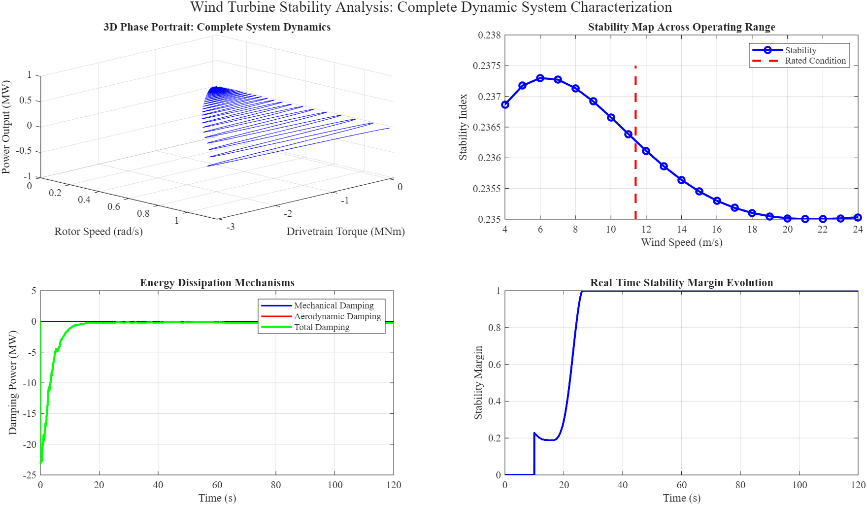
Figure 10: Full dynamic system characterization of a wind turbine. (a) A three-dimensional phase portrait that displays the simultaneous evolution of power output, drivetrain torque, and rotor speed. (b) A stability map with rated conditions noted that displays the stability index against wind speed across the operating range. (c) Energy dissipation methods displaying total damping power, aerodynamic damping, and mechanical damping with time. (d) The evolution of the stability margin in real time, which illustrates how the margin constantly changes as operational conditions change.

For working engineers, the message is very obvious. Create good models, but don’t put your blind faith in them. Whenever feasible, validate against field data. Add safety margins that take into consideration less-than-ideal outcomes. Keep an eye on how turbines behave over time, and update models when circumstances change. Above all, keep in mind that stability is a dynamic, ongoing process rather than a static state that may be confirmed once and then forgotten.

10. Conclusion

This project has shown that wind turbine stability is not a static condition that can be confirmed by steady-state calculations alone, but rather is essentially a continual dynamic process. Several important insights have been discovered through the creation and implementation of an extensive MATLAB simulation framework that includes aerodynamic disturbances, drivetrain dynamics, control systems, and grid interactions. Short-duration torque fluctuations are absorbed by the rotor inertia, which gives pitch control the time frame it needs to react to turbulence and gusts. However, when excitation frequencies coincide with natural frequencies, lightly-damped drivetrain torsional modes can amplify some disturbances by a factor of three to five, which explains why seemingly minor periodic disturbances can result in notable oscillation expansion. Control systems influence stability results in ways that heavily rely on tuning; aggressive settings shorten the settling period but increase overshoot and may completely destabilize the loop when gains beyond ideal values. The mechanical torque transients caused by grid-side disturbances, especially low-voltage ride-through events and frequency variations, can reach two to three times rated torque, proving that electrical defects have mechanical repercussions that need to be taken into account when designing a drivetrain. In comparison to idealized models, non-ideal phenomena like as sensor noise, actuator delays, and structure aging reduce stability margins by 15 to 20 percent, underscoring the significance of ongoing model improvement utilizing field measurement data. The main finding is that, in order to maintain safe and dependable performance under continuously changing conditions, stability analysis cannot be a one-time calculation done during design and then forgotten; rather, it requires continuous validation, parameter updates, and control tuning throughout the turbine’s operational life.

References

[1] T. Burton, N. Jenkins, D. Sharpe, and E. Bossanyi, Wind Energy Handbook, 2nd ed. Chichester, UK: Wiley, 2011.

[2] J. F. Manwell, J. G. McGowan, and A. L. Rogers, Wind Energy Explained: Theory, Design and Application, 2nd ed. Chichester, UK: Wiley, 2009.

[3] M. O. L. Hansen, Aerodynamics of Wind Turbines, 3rd ed. London, UK: Routledge, 2015.

[4] J. Jonkman, S. Butterfield, W. Musial, and G. Scott, “Definition of a 5-MW Reference Wind Turbine for Offshore System Development,” National Renewable Energy Laboratory, Golden, CO, Technical Report NREL/TP-500-38060, 2009.

[5] S. Heier, Grid Integration of Wind Energy: Onshore and Offshore Conversion Systems, 3rd ed. Chichester, UK: Wiley, 2014.

[6] E. A. Bossanyi, “The design of closed loop controllers for wind turbines,” Wind Energy, vol. 3, no. 3, pp. 149-163, 2000.

[7] M. H. Hansen, “Improved modal dynamics of wind turbines to avoid stall-induced vibrations,” Wind Energy, vol. 6, no. 2, pp. 179-195, 2003.

[8] S. M. Muyeen, M. Hasan, R. Takahashi, et al., “Transient stability analysis of wind generator by using six-mass drive train model,” in Proceedings of the International Conference on Electrical Machines and Systems, 2006.

[9] V. A. Riziotis, S. G. Voutsinas, E. S. Politis, and P. K. Chaviaropoulos, “Aeroelastic stability of wind turbines: the problem, the methods and the issues,” Wind Energy, vol. 7, no. 4, pp. 373-392, 2004.

[10] E. A. Bossanyi, “Wind turbine control for load reduction,” Wind Energy, vol. 6, no. 3, pp. 229-244, 2003.

[11] International Electrotechnical Commission, “IEC 61400-1: Wind energy generation systems – Part 1: Design requirements,” IEC, Geneva, Switzerland, 2019.

[12] J. C. Kaimal, J. C. Wyngaard, Y. Izumi, and O. R. Coté, “Spectral characteristics of surface-layer turbulence,” Quarterly Journal of the Royal Meteorological Society, vol. 98, no. 417, pp. 563-589, 1972.

[13] R. B. Stull, An Introduction to Boundary Layer Meteorology. Dordrecht, Netherlands: Kluwer Academic Publishers, 1988.

[14] A. L. Rogers and J. F. Manwell, “Wind shear and its effect on turbine power production,” Renewable Energy Research Laboratory, University of Massachusetts, Amherst, Technical Report, 2004.

[15] R. J. Barthelmie, S. T. Frandsen, M. N. Nielsen, et al., “Modelling and measurements of power losses and turbulence in large wind farms,” in Proceedings of the European Wind Energy Conference, Athens, Greece, 2006.

[16] L. J. Vermeer, J. N. Sørensen, and A. Crespo, “Wind turbine wake aerodynamics,” Progress in Aerospace Sciences, vol. 39, no. 6-7, pp. 467-510, 2003.

[17] D. J. Dolan and P. W. Lehn, “Simulation model of wind turbine 3p torque oscillations due to tower shadow and wind shear,” IEEE Transactions on Energy Conversion, vol. 21, no. 3, pp. 717-724, 2006.

[18] J. G. Leishman, “Dynamic stall experiments on the NACA 23012 aerofoil,” Experiments in Fluids, vol. 9, no. 1, pp. 49-58, 1990.

[19] D. J. P. M. G. L. M. M. Peeters, “Analysis of wind turbine drivetrain dynamics using multibody simulation,” Journal of Physics: Conference Series, vol. 75, no. 1, p. 012065, 2007.

[20] Z. Xu and Z. Pan, “Influence of different flexible drive train models on the transient responses of DFIG wind turbine,” in Proceedings of the 2011 International Conference on Electrical Machines and Systems, pp. 1-6, 2011.

[21] A. D. Hansen and G. Michalke, “Fault ride-through capability of DFIG wind turbines,” Renewable Energy, vol. 32, no. 9, pp. 1594-1610, 2007.

[22] W. T. Thomson and M. D. Dahleh, Theory of Vibration with Applications, 5th ed. Upper Saddle River, NJ: Prentice Hall, 1998.

[23] M. H. Hansen, “Aeroelastic stability analysis of wind turbines using an eigenvalue approach,” Wind Energy, vol. 7, no. 2, pp. 133-143, 2004.

[24] F. M. L. P. P. J. M. P. J. M. Peeters, “Investigation of the modal interaction in wind turbines using a multibody simulation approach,” in Proceedings of the International Conference on Noise and Vibration Engineering, Leuven, Belgium, 2006.

[25] P. J. Tavner, J. Xiang, and F. Spinato, “Reliability analysis for wind turbines,” Wind Energy, vol. 10, no. 1, pp. 1-18, 2007.

[26] S. S. Yang, C. Zhu, Y. Zhou, C. Li, H. Song, and B. Liao, “Dynamics modeling and analysis of a novel fully integrated wind turbine drivetrain considering aeroelastic-mechatronic-rigid-flexible coupling effects,” Ocean Engineering, vol. 341, Part 4, p. 122755, 2025.

[27] L. C. Henriksen, M. H. Hansen, and N. K. Poulsen, “A simplified model for a wind turbine with aerodynamic damping,” in Proceedings of the 2012 American Control Conference, pp. 4945-4950, 2012.

[28] C. L. Bottasso and F. Campagnolo, “Nonlinear analysis of wind turbines for design and control,” Journal of Physics: Conference Series, vol. 1037, no. 3, p. 032010, 2018.

[29] I. Razzhivin, A. Suvorov, and R. Ufa, “Development of automatic pitch angle control mathematical model for type-4 wind turbines specialized hybrid processor,” Przeglad Elektrotechniczny, vol. 97, no. 4, pp. 60-65, 2021.

[30] E. A. Bossanyi, “Controller design for wind turbines,” in Wind Energy Engineering, P. Veers, Ed. New York: Springer, 2012.

[31] M. Singh and S. Santoso, “Dynamic models for wind turbines and wind power plants,” National Renewable Energy Laboratory, Golden, CO, Technical Report NREL/TP-5500-52708, 2011.

[32] P. Pourbeik, “Generic dynamic models for modeling wind power plants and other renewable technologies in large-scale power system studies,” IEEE Transactions on Energy Conversion, vol. 32, no. 3, pp. 1108-1116, 2017.

[33] J. Morren, S. W. H. de Haan, W. L. Kling, and J. A. Ferreira, “Wind turbines emulating inertia and supporting primary frequency control,” IEEE Transactions on Power Systems, vol. 21, no. 1, pp. 433-434, 2006.

[34] E. ON Netz GmbH, “Grid Code: High and Extra High Voltage,” E. ON Netz, Bayreuth, Germany, 2006.

[35] M. P. Kazmierkowski and L. Malesani, “Current control techniques for three-phase voltage-source PWM converters: A survey,” IEEE Transactions on Industrial Electronics, vol. 45, no. 5, pp. 691-703, 1998.

[36] A. Ellis, P. Pourbeik, J. J. Sanchez-Gasca, J. Senthil, and J. Weber, “Generic wind turbine generator models for WECC – A second status report,” in Proceedings of the 2015 IEEE Power Engineering Society General Meeting, pp. 1-5, 2015.

You can download the Project files here: Download files now. (You must be logged in).