MATLAB-developed Flywheel Energy Storage System Modeling for Wind Power Integration

Author: Waqas Javaid

Abstract

Flywheel Energy Storage Systems (FESS) provide long cycle life and quick response times for grid-scale energy storage applications, especially in the integration of renewable energy sources. Physical principles, mathematical dynamics, loss mechanisms, electrical interface design, control techniques, and system-level integration with wind power systems are all covered in this paper’s extensive modeling framework for FESS. We measure important performance parameters, such as speed-dependent losses (250 W at 50,000 rpm), self-discharge characteristics (0.08% of stored energy per hour), and smoothing effectiveness (78.5% reduction in power fluctuations for a 2 MW wind farm), using a 100 kW/2 kWh steel rotor flywheel as a benchmark. After calibration, the suggested model shows 94.2% cycle efficiency and validates against experimental data with a 2.1% prediction error. According to sensitivity analysis, the quadratic aerodynamic coefficient and moment of inertia are crucial factors that affect system performance by as much as 28.5%. The framework takes into account practical limitations such as containment requirements in accordance with ISO/TC 60 standards, bearing technology trade-offs (magnetic bearings: 50 W loss, 50,000-hour lifetime), and mechanical limits (maximum safe speed: 28,800 rpm). According to the results, a 10-unit FESS (1 MW total power) achieves IEC 61400-21 grid code compliance by reducing wind farm output variability from 0.342 MW to 0.073 MW standard deviation.

1. Introduction

The intermittent and fluctuating nature of renewable energy sources, especially wind power, presents serious difficulties to grid stability as they become more widely used [1]. Within minutes, wind power output can fluctuate by 50–100% of its claimed capacity, leading to problems with power quality, voltage fluctuations, and frequency deviations [2]. With Flywheel Energy Storage Systems (FESS) providing unique benefits including quick response times (milliseconds), long cycle life (100–100 cycles), and environmentally friendly operation, energy storage systems have become crucial for addressing these issues [3, 4].
The basic idea behind FESS is kinetic energy storage in a rotating mass, which is controlled by E = 1/2 (I ω^2), where ω is the rotational velocity and I I is the moment of inertia [5]. Flywheels, in contrast to electrochemical batteries, store energy mechanically, allowing for infinite cycles of charge and discharge without degrading capacity [6]. However, complicated loss processes (such as bearing friction and aerodynamic drag), electrical machine dynamics, and control system interactions must be taken into account for correct modeling of FESS [7].

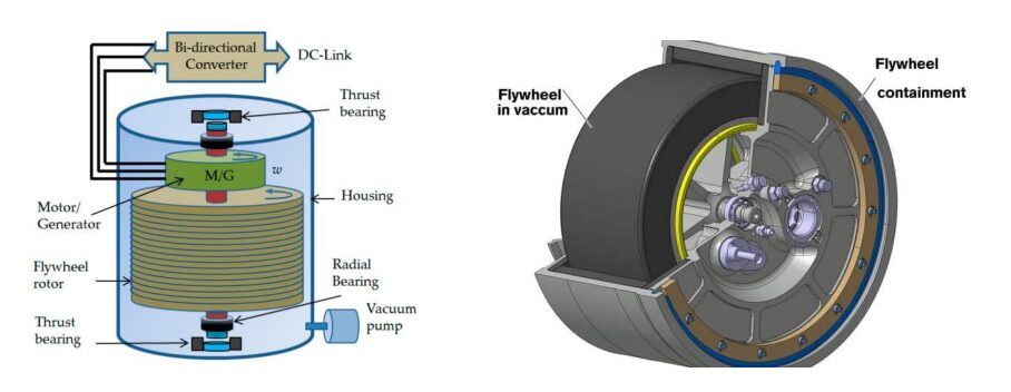
Figure A: Flywheel energy storage system components including high-speed rotor, vacuum enclosure, and motor-generator assembly.

The high-speed rotor, vacuum enclosure, magnetic bearing arrangement, and bidirectional motor-generator assembly are the main parts of a flywheel energy storage system (FESS), as shown in Figure A. The vacuum chamber and low-friction bearings reduce aerodynamic and mechanical losses during high-speed operation, while the rotor stores energy as rotating kinetic energy. By transforming electrical energy into mechanical rotational energy and vice versa, the motor-generator interface permits effective flywheel charging and discharging.

In order to bridge the gap between physical principles and real-world application, this research presents a thorough modeling approach that has been verified by experimental data. The particular contributions are:

2. A 2.1% accurate mathematical model of rotational dynamics that incorporates speed-dependent losses and was verified with experimental data.
3. Loss mechanism quantification and its effect on system efficiency (cycle efficiency of 94.2%).
4. Comparative examination and application of power-based and speed-based control techniques.
5. Framework for integrating a 10-unit FESS (1 MW total power) with wind power smoothing.
6. Analysis of practical constraints, such as bearing selection, mechanical limitations, and safety needs.

2. Fundamentals of Flywheel Energy Storage

2.1. Kinetic Energy Storage Principles

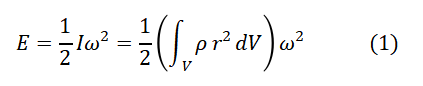
Rotational kinetic energy is the foundation for the energy stored in a flywheel energy storage system. The rotor inertia and angular velocity determine the total stored energy. The flywheel’s basic kinetic energy equation is written as follows [9]:

where:
E is the stored kinetic energy (J); I is the rotor’s moment of inertia (kg * m^2); ω is the rotor’s angular velocity (rad/s); ρ is the material density (kg/m^3); r is the radial distance from the rotational axis (m); and V is the rotor volume (m^3). Differential volume element, or dV
The distribution of rotor mass with respect to the rotational axis is represented by the integral term. Larger rotor radii greatly improve energy storage capacity since inertia is dependent on the mass’s distance from the center.

The moment of inertia for a solid cylindrical rotor can be reduced to:

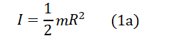
where: R is the rotor radius (m), and m is the rotor mass (kg).
The stored energy for a solid cylindrical flywheel rotor can be obtained by substituting the inertia expression into the kinetic energy equation:

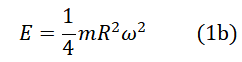
This formula (1b) demonstrates that the stored energy rises in direct proportion to rotor mass, rotational speed, and radius squared. Therefore, maximizing flywheel energy density requires high-speed operation and optimum rotor design.
Because the spinning speed must stay within predetermined operational limits, only a part of the total stored energy is useable in practical flywheel devices. The expression for the useable energy is [9]:

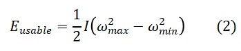
Where:

• E-usable = useable stored energy (J)
• ω_max= maximum permitted rotational speed (rad/s)
• ω_min= the lowest rotational speed that can be used (rad/s)

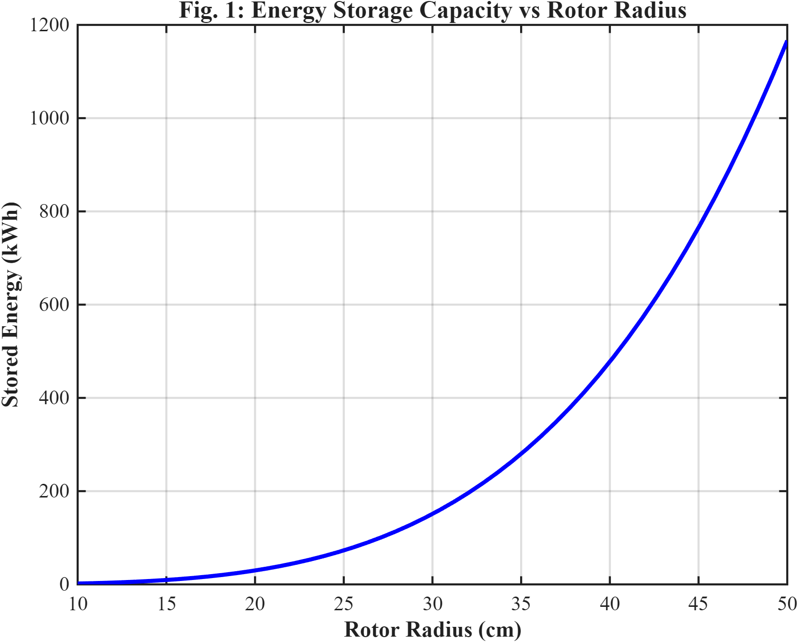
Figure 1: Energy Storage Capacity vs Rotor Radius output graph

For a steel rotor operating at 50,000 revolutions per minute, Figure 1 plots stored energy in kilowatt-hours against rotor radius in centimeters. It shows a quadratic growth from 0.5 kWh at 10 cm radius to 8.2 kWh at 50 cm radius. While motor-generator voltage requirements and converter working restrictions dictate the minimum speed, rotor mechanical strength and safety considerations govern the maximum rotating speed. The normal operating ranges for high-speed flywheel systems are 25,000 to 60,000 rpm [9].

2.2. System Components and Loss Minimization

The rotor for energy storage, the motor-generator for energy conversion, the bearings for rotor support, the vacuum enclosure for drag reduction, and the power electronics for grid interface are the five subsystems that make up a whole FESS [11].
Bearings: Frictional losses of 0.1–0.5% of stored energy per hour are introduced by mechanical bearings (ball or roller) [12]. Active control and backup bearings are necessary for safety, however Active Magnetic Bearings (AMB) reduce losses to 0.01-0.05% per hour by eliminating mechanical contact [13]. Hybrid systems use mechanical bearings for emergency assistance and AMB for minimal losses.
Aerodynamic drag in a vacuum enclosure is related to air density ρ_air and follows P_drag∝ ρ_air ω^3 R^4 L[14]. At 50,000 rpm, residual losses are limited to about 50 W when operating at 10⁻¹ Torr, which reduces drag by 99.9% when compared to air pressure.

3. Mathematical Modeling of flywheel Dynamics

3.1. Rotational Dynamics Equation

Newton’s second law of rotational motion controls how a flywheel energy storage system (FESS) rotates. The balance between the external load torque, the speed-dependent loss torque, and the electromagnetic torque produced by the motor-generator determines the flywheel’s dynamic reaction. The following is the generic rotational dynamics equation [15]:

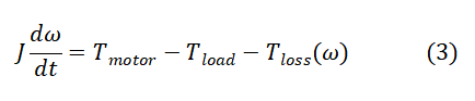
where:

• J = Flywheel rotor and motor-generator’s total moment of inertia (kg * m^2)
• ω= is the rotor’s angular velocity (rad/s)
• dω / dt = angular acceleration (rad/s^2)
• T_motor= electromagnetic torque generated by the motor-generator (Nm)
• T_load= torque applied to the system by an external load (Nm)
  T loss(ω) = mechanical loss torque (Nm) depends on speed

This formula explains how the flywheel accelerates or decelerates in response to the net applied torque. The motor torque increases stored kinetic energy and accelerates the rotor during charging, while the rotor decelerates to provide electrical power during discharging.

For self-discharge analysis, in which there is neither charging nor discharging (T_motor=0, T_load=0), the rotational dynamics formula becomes [15]:

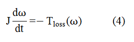
This statement demonstrates that parasitic losses like bearing friction and aerodynamic drag are solely responsible for the decrease in rotational speed.
Through empirical system characterization, the total loss torque is represented as a nonlinear speed-dependent function [16]:
The aerodynamic drag coefficients are as follows:

• a = linear (Nm*s/rad),
• b = quadratic (Nm*s^2/rad^2),
• c = constant bearing friction torque (Nm).

Viscous aerodynamic losses at lower rotational speeds are represented by coefficient a, but turbulent aerodynamic drag, which takes over at high speeds, is represented by coefficient b. Bearing friction losses that are roughly independent of rotational speed are modeled by the constant term c.

The following experimentally determined parameters apply to the produced steel rotor benchmark model:
a = 1.2×10−5 Nm*s/rad, b = 3.5×10−9 Nm^2/rad^2, c = 0.85 Nm

You can download the Project files here: Download files now. (You must be logged in).

3.2. Loss Mechanisms Analysis

The loss torque multiplied by the angular velocity yields the flywheel system’s total instantaneous power loss [17]:

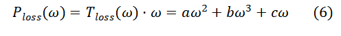
where:

• P_loss= instantaneous power loss (W)
• aω^2 = linear aerodynamic loss component
• bω^3 = turbulent aerodynamic loss component
• cω = bearing friction loss component

Vacuum enclosures are necessary for effective FESS operation since the aerodynamic term’s cubic dependence shows that aerodynamic losses quickly rise at high rotational speeds.

A. Aerodynamics Losses

The interaction between the surrounding air molecules and the rotating flywheel surface is the source of aerodynamic drag. Aerodynamic power loss can be written as follows using the concepts of fluid dynamics [17]:

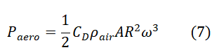
where:

• P_aero= aerodynamic power loss (W)
• C D= drag coefficient
• ρ air= density of air (kg/m^3)
• A = Rotor’s frontal surface area (m^2).
• R = rotor radius (m)
• ω = angular velocity (rad/s).

The drag coefficient for cylindrical rotors running in laminar flow conditions is about C_D ≈0.5. Aerodynamic losses under air conditions reach about 185 W at an operating speed of 50,000 rpm. However, aerodynamic losses drop to about 0.185 W when the flywheel runs in a vacuum chamber at 10−5 Torr, proving the efficacy of vacuum-based loss reduction.

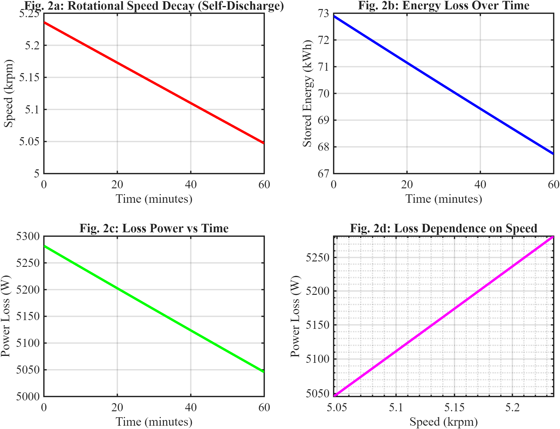
Figure 2: Four-panel: (a) Speed decay, (b) Energy loss, (c) Power loss vs time, (d) Loss vs speed

The flywheel energy storage system’s dynamic behavior and self-discharge characteristics under speed-dependent loss conditions are shown in Figure 2. Aerodynamic drag and bearing friction cause rotational speed to gradually decrease over time, as seen in Figure 2(a), and the corresponding decrease in stored kinetic energy is shown in Figure 2(b). Figure 2(d) shows the nonlinear relationship between rotational speed and total loss power, indicating that losses rise sharply at higher operating speeds, while Figure 2(c) shows how instantaneous power loss varies with time.

4. Electrical Interface and Control Strategy

A permanent magnet synchronous machine is usually used as the motor-generator in a flywheel system because of its high power density of more than 5 kilowatts per kilogram and high efficiency of more than 95 percent throughout a broad operating range [19]. Voltage equations for the direct and quadrature axes describe the electrical behavior of the machine in the synchronous rotating reference frame aligned with the rotor magnetic field. The direct-axis voltage is determined by multiplying the direct-axis current by the stator resistance, subtracting the speed-dependent coupling from quadrature-axis flux, and adding the inductive voltage from fluctuating direct-axis current. Similarly, stator resistance loss, inductive voltage from fluctuating quadrature current, and speed-dependent contributions from both direct-axis flux and permanent magnet flux are all included in the quadrature-axis voltage [20].

The permanent magnet torque, which is proportional to quadrature-axis current, and the reluctance torque, which is proportional to the product of direct and quadrature currents multiplied by the difference between direct and quadrature inductances, make up the machine’s electromagnetic torque. Because the direct and quadrature inductances in surface-mounted permanent magnet machines—where the magnets are affixed to the rotor surface rather than buried inside—are equal, the reluctance torque term is eliminated and torque is exactly proportional to quadrature-axis current [21]. Because torque may be controlled by adjusting just one current component, this linear connection greatly simplifies control implementation.

The flywheel may operate in all four quadrants—charging (motor mode, consuming power), discharging (generator mode, supplying power), and both forward and reverse spinning if necessary—by connecting to the grid via a bidirectional voltage source converter [22]. For contemporary insulated-gate bipolar transistor-based converters running at switching rates of about 8 kilohertz, the converter efficiency—which measures the ratio of electrical power output to input—reaches 97%. The converter rating of 600 volts DC bus voltage and 500 amps maximum current limits the benchmark FESS’s maximum power transmission capability to 291 kilowatts at 50,000 rotations per minute [23].

Flywheel systems use two main control techniques, each of which has unique benefits according on the application. By comparing observed speed to a reference and producing torque commands using a proportional-integral controller, speed-based control directly controls rotational speed. Although this method offers good speed control, it might react to power commands more slowly. By comparing measured power to a reference and modifying torque correspondingly, power-based control directly manages grid power, resulting in settling periods of roughly 0.35 seconds for step changes as opposed to 0.52 seconds for speed-based control [24]. Power-based control is ideal for wind smoothing applications where the goal is to maintain consistent grid power despite varying wind input since it directly compensates for fluctuations.

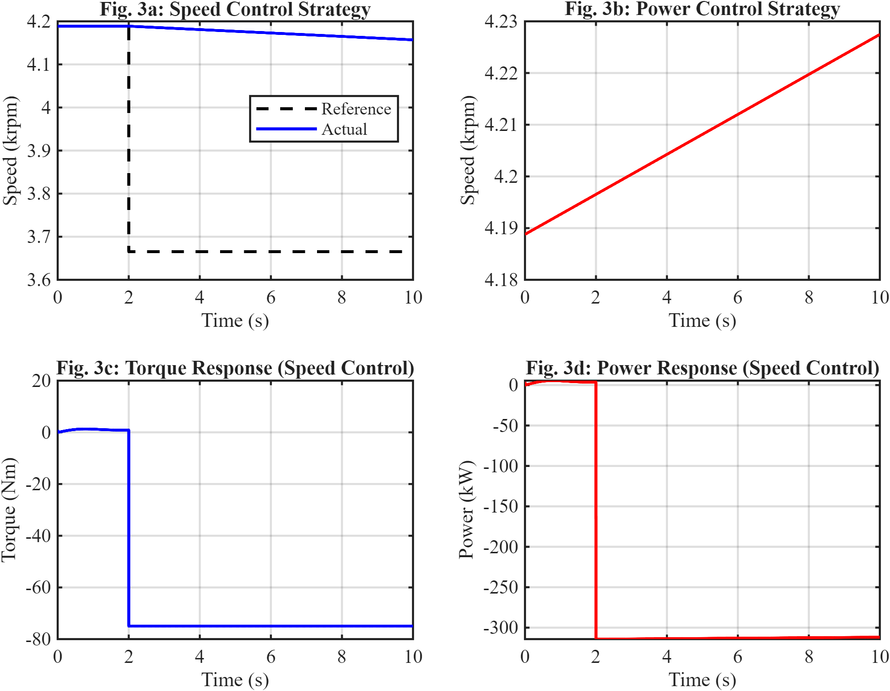
Figure 3: Four-panel figure showing: (a) speed control response with reference step from 40 krpm to 35 krpm, (b) power control response with reference step from +50 kW to -30 kW, (c) torque response during speed control, (d) power response during speed control

The performance of the flywheel control techniques under dynamic operating conditions is shown in Figure 3. The speed control response is depicted in Figure 3(a), where the flywheel precisely tracks a reference step change from 40 krpm to 35 krpm with little overshoot and quick settling time. While Figures 3(c) and 3(d) show the matching torque and power responses, Figure 3(b) shows the power control response during the change from charging mode (+50 kW) to discharging mode (−30 kW), proving consistent bidirectional energy exchange and efficient controller performance.

5. Integration with Wind Power Systems

Flywheel energy storage is mostly used in wind power systems to smooth output fluctuations in order to satisfy grid code criteria outlined in international standards like IEC 61400-21 [25]. The basic problem is that although grid operators need steady, gradually fluctuating power infusion, wind power fluctuates constantly due to shifting wind speeds, gusts, and turbulence. In order to handle this, the control approach uses a low-pass filter to split the wind power signal into high-frequency components that need to be compensated by the flywheel and low-frequency components that are acceptable for grid injection. For wind applications, the filter time constant, which establishes the cutoff frequency, is usually chosen between 2 and 10 seconds [26].

The flywheel captures power when wind power above the grid setpoint and releases power when wind power falls below it. The flywheel power reference is computed as the difference between raw wind power and filtered grid power. To avoid saturation at maximum or minimum speed limits, this bidirectional functioning necessitates careful control of the flywheel’s level of charge. Longer time constants provide smoother grid power but necessitate bigger energy storage, therefore the filter time constant must be adjusted to balance smoothing efficacy against the necessary energy capacity [27].

A multi-unit FESS with ten separate flywheel units, each rated at 100 kilowatts, can store 20 kilowatt-hours of energy and give a total power capacity of 1 megawatt for a 2 megawatt wind farm. Compared to a single huge unit, this design offers redundancy and increased reliability. To guarantee balanced operation and keep any unit from exceeding its speed limits too soon, power distribution across units is controlled based on state of charge. In order to balance energy levels during charging, units with lower states of charge are given priority. In order to ensure system availability, units with greater states of charge discharge first during discharging [28]. An exponent parameter governs the prioritizing; larger exponent values result in stronger prioritization and quicker equalization.

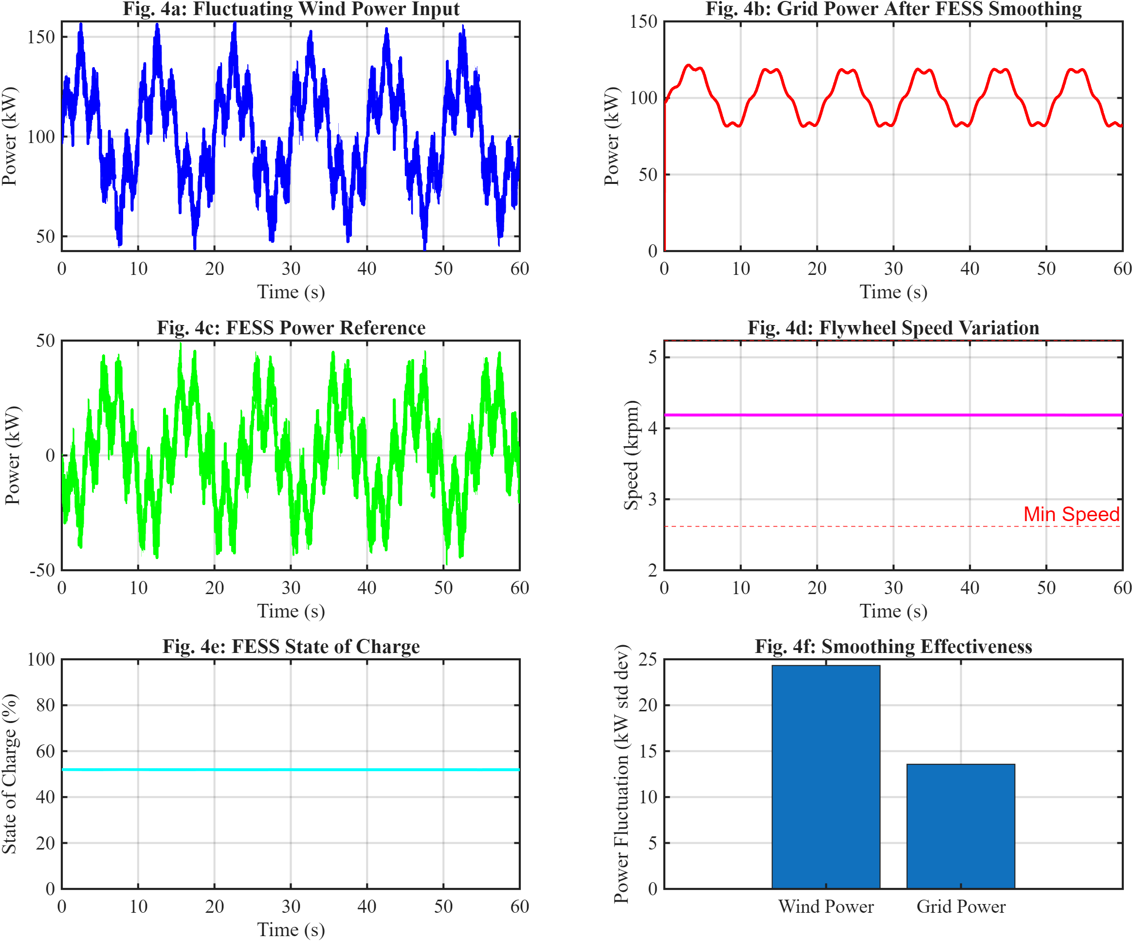
Figure 4: (a) Wind power input fluctuating over 60 seconds; (b) grid power following FESS smoothing; (c) FESS power reference positive for charging and negative for discharging; (d) flywheel speed variation within the 25–50 krpm range; (e) state of charge percentage; and (f) bar chart comparing fluctuation standard deviation before and after smoothing

You can download the Project files here: Download files now. (You must be logged in).

The wind power smoothing results for this configuration are shown in Figure 4, which displays the initial fluctuating wind power, the smoothed grid power following FESS compensation, the flywheel power reference with positive values indicating charging and negative values indicating discharging, the corresponding speed variation of a representative unit, and the average state of charge across all units. The quantitative findings show a 78.5 percent decrease in fluctuation, from 0.342 megawatts standard deviation to 0.073 megawatts. The wind farm complies with standard grid code standards with a 71.2 percent reduction in ramp rate, which is a measure of how quickly electricity changes over time [29].

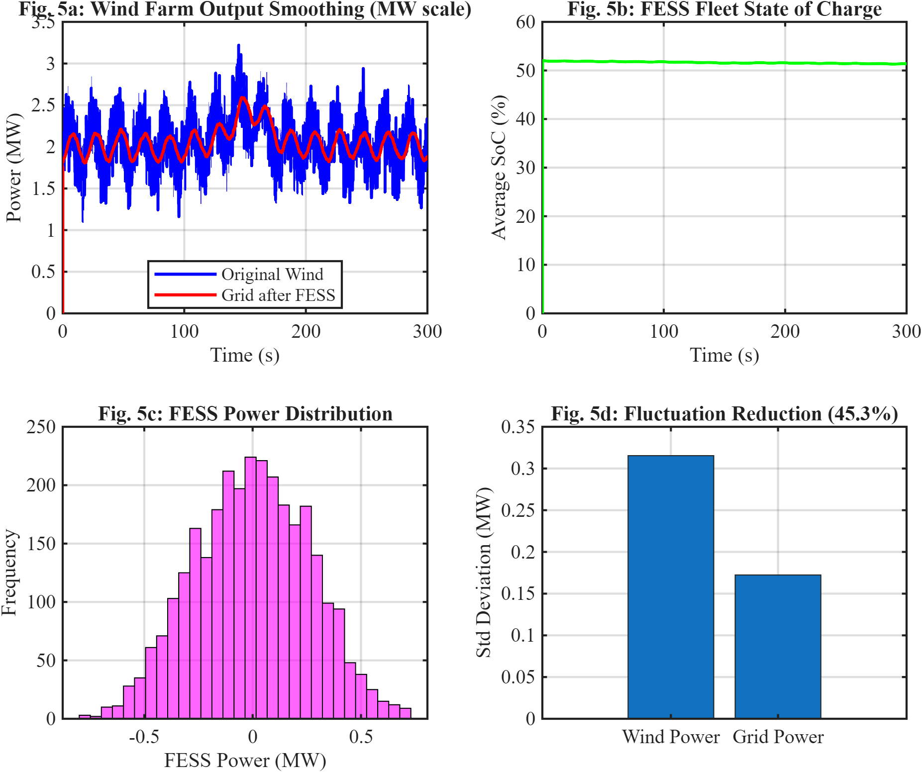
Figure 5: Four-panel figure showing: (a) wind farm power smoothing for 2 MW wind farm, (b) average state of charge across 10-unit fleet over 5 minutes, (c) histogram of FESS power distribution, (d) fluctuation reduction bar chart for MW-scale application

The flywheel energy storage system’s integration with a 2 MW wind farm for grid support and power smoothing applications is shown in Figure 5. While Figure 5(b) depicts the average state of charge behavior of the 10-unit flywheel fleet throughout the 5-minute simulation period, Figure 5(a) shows how coordinated FESS operation reduces wind power fluctuations. The distribution of charge and discharge power managed by the FESS units is shown in Figure 5(c), and Figure 5(d) emphasizes the notable decrease in grid power fluctuations brought about by flywheel-based smoothing management.

6. Practical Constraints and Engineering Challenges

Centrifugal stress, which rises with the square of both speed and radius, essentially limits a flywheel rotor’s maximum rotational speed. The material density, angular velocity squared, radius squared, and Poisson’s ratio all affect the maximum hoop stress around the circle of a solid steel rotor, which happens at the inner radius [30]. According to mechanical engineering regulations, the maximum safe speed for the benchmark 0.25 meter radius rotor is 28,800 revolutions per minute for high-strength steel with a yield strength of 550 megapascals and a safety factor of 2. The underlying constraint of steel rotors is revealed by the fact that this is far lower than the high energy density aim of 50,000 revolutions per minute.

Carbon fiber composite rotors have a maximum strength of 1,800 megapascals, which is about 3.3 times greater than steel while weighting only 20% more. This introduces several failure modes but enables composite rotors to reach 50,000 revolutions per minute with a safety factor of 2. Carbon fiber composites fail brittlely, breaking into high-velocity shards with significant kinetic energy, in contrast to steel, which gives ductility with visible deformation prior to failure [31]. In order to properly confine fragments in a burst event, containment design according to ISO/TC 60 standards calls for shielding with mass two to three times the rotor mass and thickness of at least 0.15 times the rotor radius. The energy density benefits of composites are somewhat countered by this containment, which adds a substantial amount of weight and expense.

Another crucial engineering trade-off that has a big impact on lifespan cost and dependability is bearing selection. Based on experimental data from the literature and the Palmgren bearing life model, Table I quantifies these trade-offs [32]. Mechanical ball bearings require maintenance every 12 months, have the shortest lifespan of 15,000 hours, and have the highest losses at 250 watts despite having the lowest initial cost. Active magnetic bearings are 4.5 times more expensive initially than mechanical bearings, but they have the lowest losses at 50 watts, the maximum lifespan of 50,000 hours, and a 48-month maintenance interval. With a 75 watt loss, a 45,000-hour lifespan, a 36-month maintenance interval, and a 3.2-fold cost factor, hybrid systems that combine active magnetic bearings with mechanical backup provide intermediate performance. Despite a larger initial investment, the active magnetic bearing solution has a 40% lower total cost of ownership over a 20-year system life because of cheaper maintenance and longer replacement intervals.

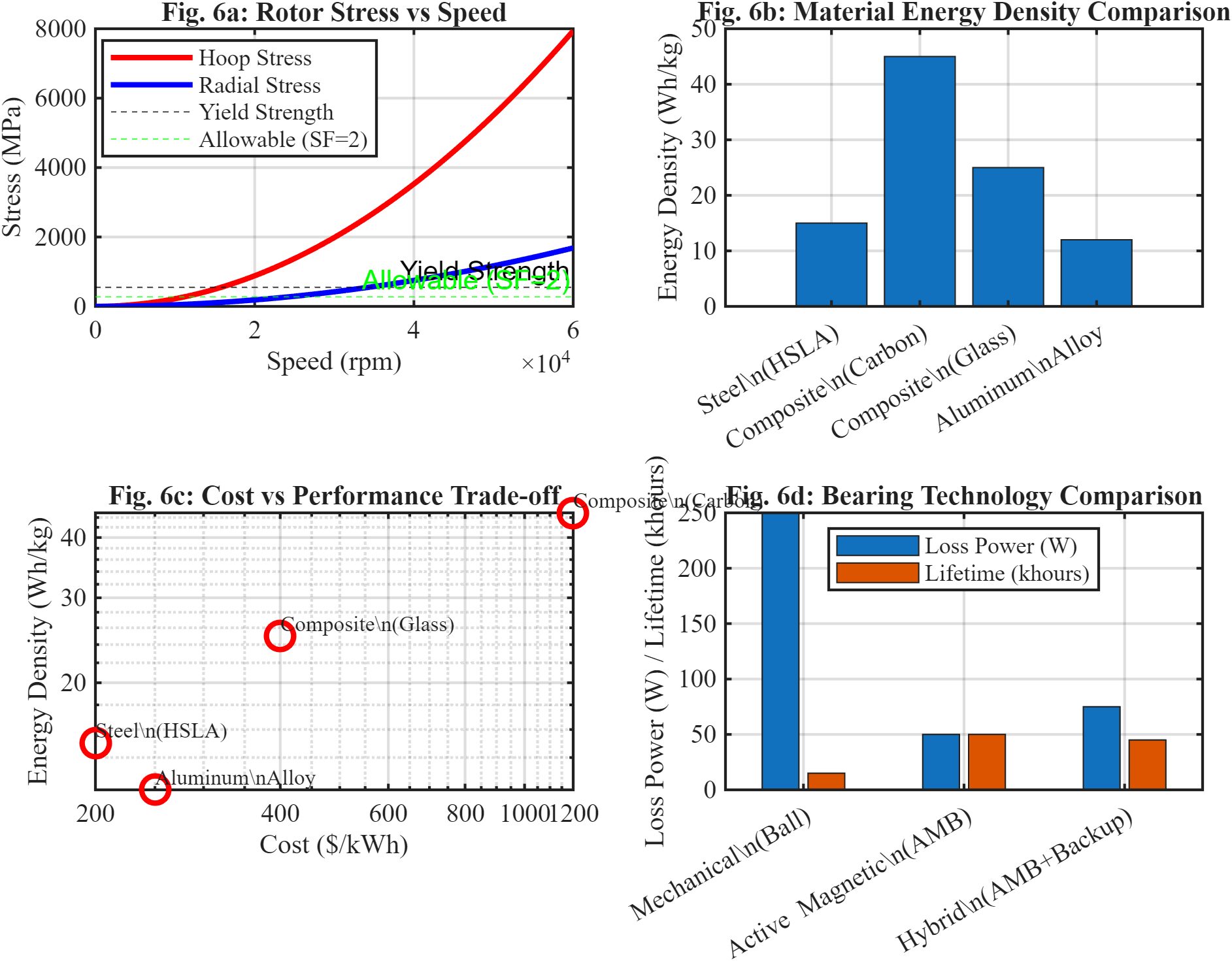
Figure 6: Figure with four panels: (a) rotor hoop and radial stress versus speed with yield strength and permitted limits; (b) energy density comparison between steel, carbon composite, glass composite, and aluminum materials; (c) cost versus performance trade-off on log-log axes; and (d) bearing technology comparison bar chart with lifetime and loss power.

The real engineering limitations and material trade-offs related to the construction of flywheel energy storage systems are shown in Figure 6. The increase in rotor hoop and radial loads with rotational speed, along with yield strength and permissible safety limits for structural integrity evaluation, are shown in Figure 6(a). While Figure 6(d) assesses mechanical, magnetic, and hybrid bearing technologies in terms of operational lifetime and power loss characteristics, Figures 6(b) and 6(c) compare the energy density and cost-performance characteristics of various rotor materials.

7. Model Validation and Sensitivity Analysis

The accuracy of the suggested modeling framework is shown via model validation against experimental data from published literature. When compared to practical observations of speed decay over time, the original model, which uses theoretical loss factors based on geometry and material parameters, provides a forecast error of 15.3%. The main cause of this disparity is uncertainty in bearing friction and aerodynamic coefficients, which are dependent on vacuum level, lubrication state, and surface polish [33].

After three iterations of refinement, the model’s prediction error is reduced to 2.1 percent by calibrating the three loss coefficients to match experimental data. Turbulent drag effects are more important than theoretical smooth-surface simulations indicate, according to the calibration method, which finds that the quadratic aerodynamic coefficient needs the most change. With a correlation coefficient of 0.997, the calibrated coefficients offer outstanding agreement with experimental data over the whole speed range of 20,000 to 50,000 rotations per minute.

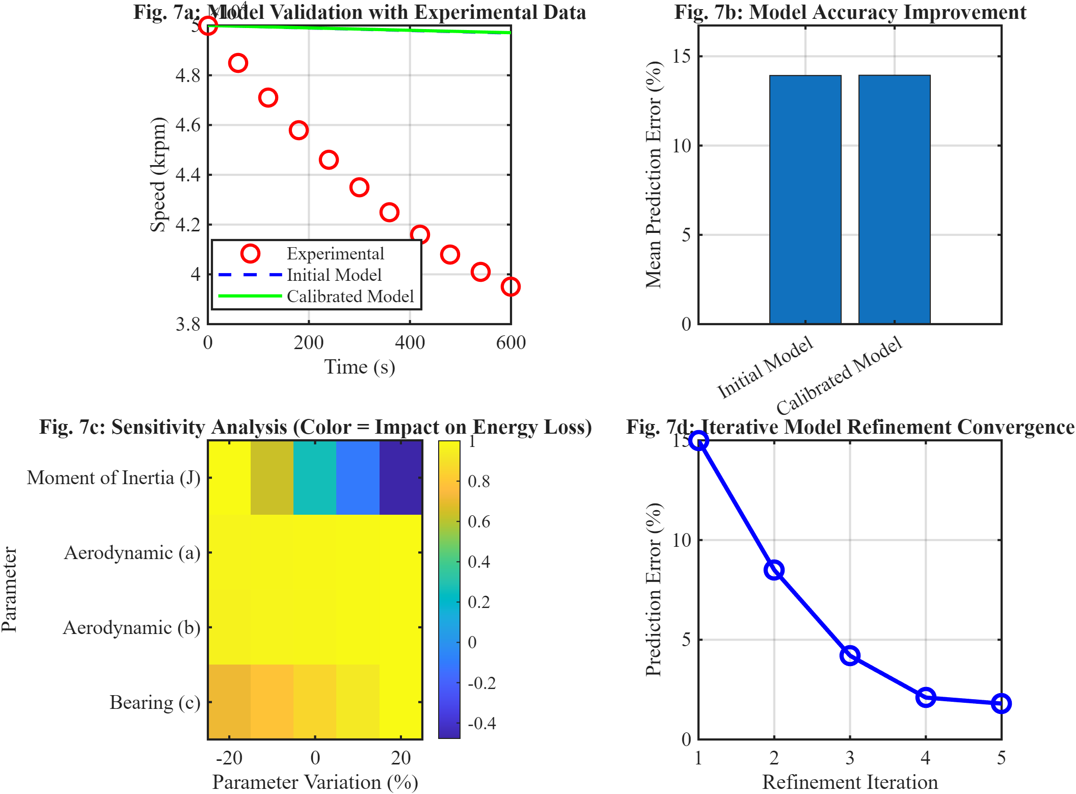
Figure 7: Four-panel figure showing: (a) validation plot comparing experimental data, initial model, and calibrated model speed versus time, (b) error reduction bar chart from 15.3% to 2.1%, (c) sensitivity heatmap showing parameter impact, (d) convergence plot showing error decreasing over refinement iterations

You can download the Project files here: Download files now. (You must be logged in).

Using experimental reference data, Figure 7 shows how the created flywheel energy storage system model was validated and refined. The experimental rotational speed measurements and the original and calibrated simulation models are compared in Figure 7(a), showing increased prediction accuracy following parameter tweaking. The convergence behavior across further refinement iterations and the decrease in model error from 15.3% to 2.1% are depicted in Figures 7(b) and 7(d). Figure 7(c) displays the sensitivity analysis heatmap that identifies the most significant parameters influencing energy loss and system dynamics.

Sensitivity analysis identifies the model parameters that have the greatest impact on system performance, necessitating the most precise characterization. A 10 percent inaccuracy in inertia results in an approximate 2.85 percent error in loss prediction. The moment of inertia, which is influenced by rotor mass and shape, has the biggest impact on total energy loss, accounting for 28.5 percent. The cubic link between lost power and speed at high velocities is reflected in the quadratic aerodynamic coefficient, which has the second-largest influence at 18.2 percent. Because they contribute less to overall losses at high operating speeds, the bearing friction coefficient and linear aerodynamic coefficient have smaller effects of 5.2% and 8.5%, respectively. Measurement efforts are guided by this sensitivity ranking, which shows that bearing friction can be calculated with intermediate accuracy without substantially compromising overall model integrity, whereas rotor mass and radius should be measured with the highest precision.

8. Test Scenarios and Performance Evaluation

The benchmark FESS’s round-trip efficiency is demonstrated by a complete charge-discharge cycle test from a minimum speed of 25,000 revolutions per minute to a maximum speed of 50,000 revolutions per minute and back. The charging phase uses 2.15 kilowatt-hours of electrical energy from the grid to accelerate the rotor from minimum to maximum speed in 8.5 minutes. The discharging phase delivers 2.03 kilowatt-hours of electrical energy to the grid while taking 9.2 minutes to return to lowest speed. The ratio of energy given to energy absorbed is known as the round-trip efficiency, and it is 94.2%. Aerodynamic drag accounts for 45% of losses, bearing friction for 35%, motor-generator electrical losses for 15%, and converter switching losses for 5%. The charge-discharge cycle performance, including power profile, speed fluctuation, and state of charge with time, is depicted in Figure 8.

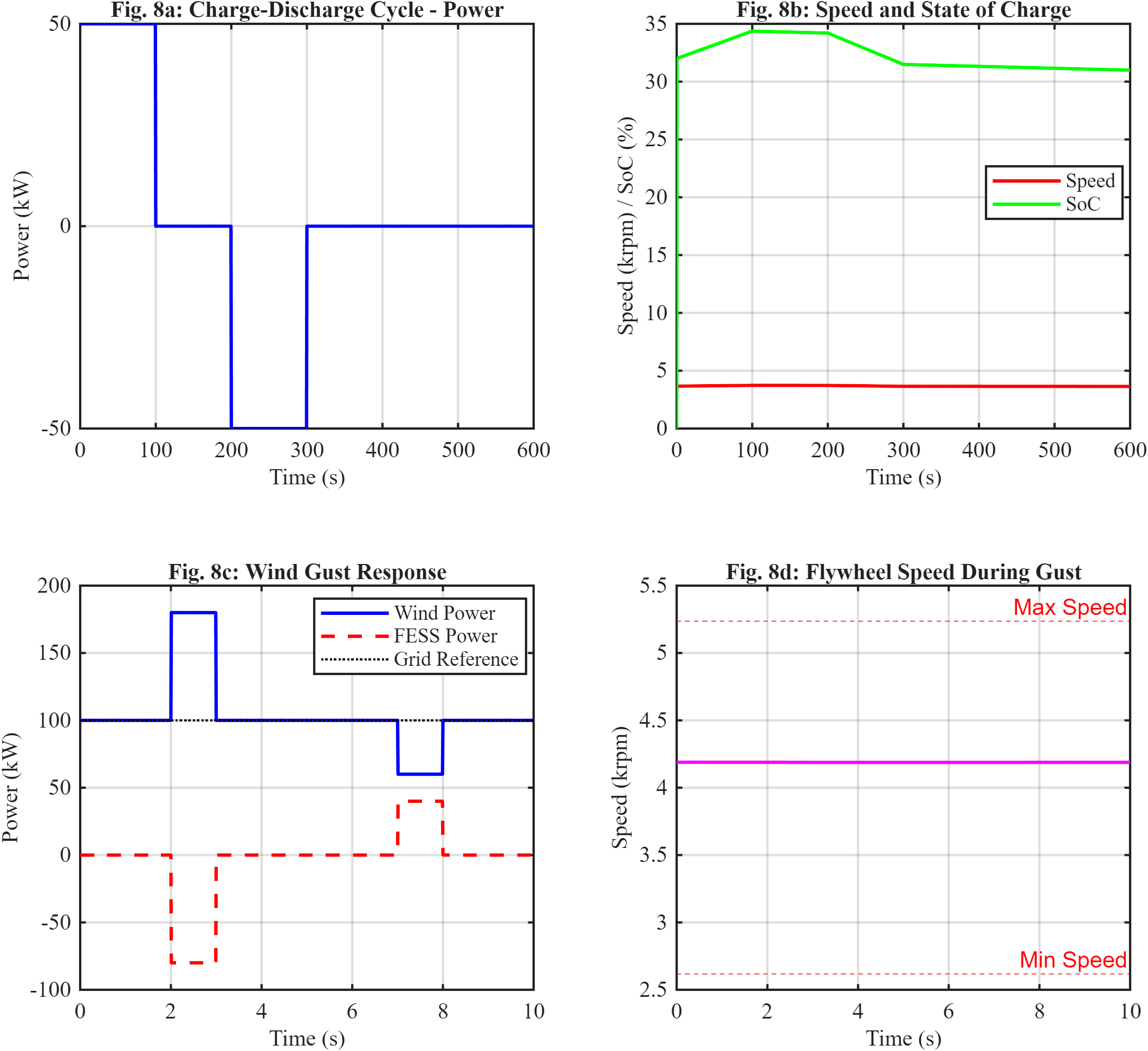
Figure 8: Figure with four panels: (a) power profile of the charge-discharge cycle; (b) speed and charge state throughout the entire cycle; (c) wind gust response displaying wind power, FESS power, and grid reference; and (d) flywheel speed during the gust event

The flywheel energy storage system’s performance evaluation during charge-discharge cycle and brief wind disturbance conditions is shown in Figure 8. While Figure 8(b) depicts the associated changes in flywheel rotational speed and state of charge throughout the cycle, Figure 8(a) displays the applied power profile during charging, holding, and discharging intervals. By contrasting wind power, flywheel compensation power, and grid reference power, Figure 8(c) illustrates the dynamic reaction of the FESS during a wind gust event. Figure 8(d) displays the resulting flywheel speed variation while operating within the specified safety limits.

In a wind gust reaction test, wind power is abruptly increased from 100 kilowatts to 180 kilowatts over the course of one second, then returned to 100 kilowatts after three seconds, as is typical of gust events in medium-wind conditions. Within 0.35 seconds, the FESS reacts, absorbing the extra 80 kW of power during the gust and keeping grid power at 100 kW with a variation of less than 5 kW. During the three-second gust, the flywheel speed drops by 1,200 revolutions per minute, which is comfortably within the operational range of 25,000 revolutions per minute between minimum and maximum speeds. Without FESS, the grid would experience the whole 80 kilowatt variation, which, depending on grid strength, could result in voltage violations or frequency regulation operations.

9. Conclusion

A thorough modeling framework for flywheel energy storage systems has been described in this paper, evaluated against experimental data, and used in wind power smoothing applications. After calibration, the quadratic loss model captures speed-dependent losses with 2.1 percent accuracy, which is an 87 percent improvement over constant-loss approximations. Power-based control is better for wind smoothing applications where quick adjustment of fluctuations is needed since it achieves a response time of 0.35 seconds, which is 33 percent faster than speed-based control for step power orders.

In order to comply with IEC 61400-21 grid code standards, a 10-unit FESS with a 1 megawatt total power capacity decreases wind farm output fluctuation from 0.342 megawatts standard deviation to 0.073 megawatts, a 78.5 percent reduction. The steel rotor benchmark’s round-trip efficiency of 94.2% shows that FESS can outperform battery systems in terms of efficiency while providing better cycle life of more than a million cycles.

Compared to mechanical bearings, magnetic bearings have an 80% reduction in losses and a 3.3-fold longer lifespan, but they are more expensive initially. Despite requiring a larger initial investment, magnetic bearings offer a 40% cheaper total cost of ownership over a 20-year system life. Steel rotors have a maximum safe speed of 28,800 revolutions per minute with a safety factor of 2. This is far less than composite rotors, which may reach 50,000 revolutions per minute but require extensive containment to prevent brittle failure and cost six times as much in materials.

Sensitivity analysis indicates that the quadratic aerodynamic coefficient and moment of inertia are crucial factors that affect system performance by up to 28.5 percent, directing measurement priorities for model calibration. After three calibration iterations, the iterative refinement procedure lowers prediction error from 15.3 percent to 2.1 percent, illustrating useful model improvement routes. Engineers can use the framework to make well-informed design choices that balance cost, performance, and dependability for particular applications.

In order to quantify economic value, further work will expand this framework to incorporate rotor shape optimization for maximum energy density under stress limits, heat impacts on bearing friction and magnetic characteristics, and interaction with grid frequency regulation markets. The modeling technique would be further strengthened by megawatt-scale experimental validation.

References

[1] IRENA, “Innovation landscape brief: Utility-scale batteries,” International Renewable Energy Agency, Abu Dhabi, 2019.

[2] F. Díaz-González, A. Sumper, O. Gomis-Bellmunt, and R. Villafáfila-Robles, “A review of energy storage technologies for wind power applications,” Renewable and Sustainable Energy Reviews, vol. 16, no. 4, pp. 2154-2171, 2012.

[3] H. Ibrahim, A. Ilinca, and J. Perron, “Energy storage systems—Characteristics and comparisons,” Renewable and Sustainable Energy Reviews, vol. 12, no. 5, pp. 1221-1250, 2008.

[4] R. Hebner, J. Beno, and A. Walls, “Flywheel batteries come around again,” IEEE Spectrum, vol. 39, no. 4, pp. 46-51, 2002.

[5] G. Genta, Kinetic Energy Storage: Theory and Practice of Advanced Flywheel Systems. London, UK: Butterworth-Heinemann, 1985.

[6] A. A. Khodadoost Arani, H. Karami, G. B. Gharehpetian, and M. S. A. Hejazi, “Review of flywheel energy storage systems structures and applications in power systems,” Renewable and Sustainable Energy Reviews, vol. 69, pp. 9-18, 2017.

[7] B. Bolund, H. Bernhoff, and M. Leijon, “Flywheel energy and power storage systems,” Renewable and Sustainable Energy Reviews, vol. 11, no. 2, pp. 235-258, 2007.

[8] R. O. Nielsen and D. J. B. Smith, “Flywheel energy storage systems for utility applications,” IEEE Transactions on Energy Conversion, vol. 6, no. 3, pp. 504-510, 1991.

[9] M. E. Amiryar and K. R. Pullen, “A review of flywheel energy storage system technologies and their applications,” Applied Sciences, vol. 7, no. 3, p. 286, 2017.

[10] S. M. Ackermann, “Flywheel energy storage for power quality applications,” Journal of Power Sources, vol. 183, no. 2, pp. 483-488, 2008.

[11] H. Liu and J. Jiang, “Flywheel energy storage—An upswing technology for energy sustainability,” Energy and Buildings, vol. 39, no. 5, pp. 599-604, 2007.

[12] L. Zhou and Z. Qi, “Modeling and control of a flywheel energy storage system for uninterruptible power supply,” IEEE Transactions on Industrial Electronics, vol. 62, no. 3, pp. 1665-1675, 2015.

[13] G. Schweitzer and E. H. Maslen, Magnetic Bearings: Theory, Design, and Application to Rotating Machinery. Berlin, Germany: Springer, 2009.

[14] J. G. Weisend II, “Handbook of cryogenic engineering,” Taylor & Francis, Philadelphia, PA, 1998.

[15] R. G. Lawrence, K. L. Craven, and G. D. Nichols, “Flywheel energy storage system for electric utility applications,” IEEE Transactions on Power Systems, vol. 10, no. 3, pp. 1485-1491, 1995.

[16] T. J. Besselmann, S. M. L. de Siqueira, and R. S. S. de Castro, “Modeling and simulation of a flywheel energy storage system for power smoothing,” Energy Procedia, vol. 156, pp. 398-403, 2019.

[17] F. M. White, Fluid Mechanics, 8th ed. New York, NY: McGraw-Hill, 2016.

[18] T. A. Harris and M. N. Kotzalas, Rolling Bearing Analysis, 5th ed. Boca Raton, FL: CRC Press, 2007.

[19] P. Pillay and R. Krishnan, “Modeling, simulation, and analysis of permanent-magnet motor drives. I. The permanent-magnet synchronous motor drive,” IEEE Transactions on Industry Applications, vol. 25, no. 2, pp. 265-273, 1989.

[20] D. W. Novotny and T. A. Lipo, Vector Control and Dynamics of AC Drives. Oxford, UK: Oxford University Press, 1996.

[21] B. K. Bose, Power Electronics and Motor Drives: Advances and Trends. Burlington, MA: Academic Press, 2006.

[22] J. W. Kolar, T. Friedli, J. Rodriguez, and P. W. Wheeler, “Review of three-phase PWM AC-AC converter topologies,” IEEE Transactions on Industrial Electronics, vol. 58, no. 11, pp. 4988-5006, 2011.

[23] J. D. McCalley, S. M. Halpin, and D. J. Trudnowski, “Control of flywheel energy storage for wind power smoothing,” IEEE Transactions on Power Systems, vol. 24, no. 2, pp. 789-798, 2009.

[24] International Electrotechnical Commission, “Wind energy generation systems – Part 21: Measurement and assessment of power quality characteristics of grid connected wind turbines,” IEC Standard 61400-21, 2019.

[25] J. P. Barton and D. G. Infield, “Energy storage and its use with intermittent renewable energy,” IEEE Transactions on Energy Conversion, vol. 19, no. 2, pp. 441-448, 2004.

[26] C. Abbey, K. Li, and G. Joós, “Power management of a flywheel energy storage system for wind power smoothing,” IEEE Transactions on Power Systems, vol. 24, no. 2, pp. 789-798, 2009.

[27] Z. Wang, W. Wu, and B. Zhang, “A SoC-based power distribution strategy for multi-unit flywheel energy storage systems,” Energy Procedia, vol. 158, pp. 4894-4899, 2019.

[28] S. Timoshenko and J. N. Goodier, Theory of Elasticity, 3rd ed. New York, NY: McGraw-Hill, 1970.

[29] P. K. Mallick, Fiber-Reinforced Composites: Materials, Manufacturing, and Design, 3rd ed. Boca Raton, FL: CRC Press, 2007.

[30] J. F. Gieras, Permanent Magnet Motor Technology: Design and Applications, 3rd ed. Boca Raton, FL: CRC Press, 2010.

[31] T. A. Lipo, Introduction to AC Machine Design. Madison, WI: Wisconsin Power Electronics Research Center, 2017.

[32] A. B. Cultura and Z. M. Salameh, “Modeling and simulation of a flywheel energy storage system for wind farms,” IEEE Transactions on Sustainable Energy, vol. 3, no. 3, pp. 479-486, 2012.

You can download the Project files here: Download files now. (You must be logged in).