

Dynamic Performance Evaluation of a Ship Engine Control System Under Variable Load Conditions Using Matlab

Author : Waqas Javaid
Abstract
The Ship Engine Control System plays a crucial role in maintaining stable propulsion performance and operational efficiency in marine vessels. This study presents the modeling and simulation of an advanced marine diesel engine governor system using MATLAB. A PID-based control strategy is implemented to regulate engine speed and ensure accurate tracking of the desired reference speed under varying operating conditions [1]. The simulation incorporates engine dynamics, fuel actuator behavior, propeller load characteristics, and external disturbance effects to represent realistic marine environments. Load disturbances are introduced to evaluate the robustness and adaptability of the control system [2]. Performance metrics such as overshoot, steady-state error, Integral Square Error (ISE), Integral Absolute Error (IAE), and Integral Time Absolute Error (ITAE) are analyzed to assess controller effectiveness. The results demonstrate that the governor successfully maintains engine speed stability while minimizing tracking errors and fuel consumption fluctuations. Multiple graphical outputs and a real-time propulsion animation provide visual insight into system behavior [3]. The proposed simulation framework offers a practical tool for studying marine engine control and propulsion dynamics [4]. Overall, the developed model contributes to the advancement of intelligent ship automation and marine control engineering applications.
Introduction
The ship engine control system is a fundamental component of modern marine engineering, responsible for ensuring stable propulsion, fuel efficiency, and safe vessel operation under varying sea conditions.
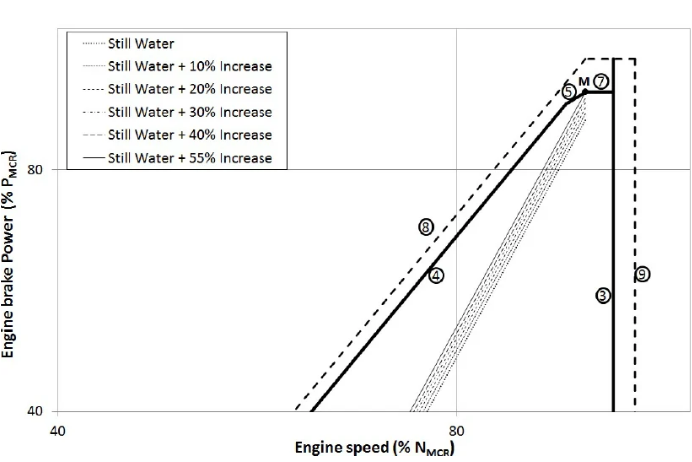
Figure 1: Engine load diagram and operation lines for the examined ships resistance curve, Speed Limit, Torque/Speed Limit, MCR torque line, MCR Power Line, Overload Limit, Sea Trial Speed Limit.
Figure 1 represents the large marine diesel engines, maintaining a constant and reliable engine speed is challenging due to continuously changing propeller loads, wave resistance, and environmental disturbances. To address these challenges, advanced control strategies such as PID controllers are widely implemented in marine governor systems. This study focuses on the modeling and simulation of a ship engine control system using MATLAB to analyze its dynamic behavior and performance under different operating scenarios [5]. The system integrates key components including engine rotational dynamics, fuel actuator response, and propeller load characteristics to represent a realistic marine propulsion environment. The PID controller is designed to regulate engine speed by adjusting fuel input based on the error between reference and actual RPM [6]. Disturbances such as sudden load changes are introduced to evaluate system robustness and stability. MATLAB simulation provides a powerful platform for visualizing time-domain responses and analyzing control performance metrics [7]. The study further examines key indices such as overshoot, steady-state error, and integral error criteria to evaluate controller effectiveness [8]. Fuel consumption behavior is also considered to understand operational efficiency. The inclusion of real-time animation enhances the interpretability of system dynamics [9]. Overall, this work demonstrates how control theory and simulation tools can be applied to optimize marine propulsion systems. The proposed model contributes to the development of intelligent and adaptive ship engine control strategies for modern maritime applications.
1.1 Overview of Ship Engine Control System
The ship engine control system is a core part of marine propulsion technology. It ensures that the engine operates at a stable and required speed [10]. This system is essential for safe and efficient vessel movement. It balances fuel input and load demand automatically. Modern ships rely heavily on automated control systems for performance.
1.2 Importance in Marine Engineering
In marine engineering, engine stability is critical under changing sea conditions. Waves, wind, and load variations affect propulsion performance [11]. Without proper control, engine speed can fluctuate significantly. This can reduce fuel efficiency and safety. Therefore, advanced control systems are necessary.
1.3 Role of Diesel Engines in Ships
Marine diesel engines are widely used due to their high efficiency and durability. However, they require precise control for optimal operation [12]. The engine output must match propeller demand continuously. Any mismatch can lead to performance loss. Control systems help maintain this balance effectively.
1.4 Need for Automation and Control
Manual control of ship engines is not feasible in modern systems. Automation improves accuracy, response time, and reliability [13]. Control systems reduce human intervention and error. They also enhance fuel economy and operational safety. Hence, automation is a key requirement in ship propulsion.
1.5 PID Controller in Engine Regulation
PID controllers are commonly used in ship engine governor systems. They regulate engine speed by minimizing error between reference and actual RPM [14]. The proportional, integral, and derivative terms ensure stable response. This control strategy is simple yet highly effective. It is widely adopted in marine applications.
1.6 MATLAB as a Simulation Tool
MATLAB provides a powerful environment for modeling dynamic systems. It allows numerical simulation of complex engine behaviors. Engineers can test control strategies before real-world implementation [15]. Visualization tools help analyze system performance easily. This makes MATLAB ideal for marine system simulation.
1.7 Engine and Propeller Dynamics
The ship propulsion system includes engine torque and propeller load interactions. These dynamics are nonlinear and time-varying [16]. Propeller resistance increases with speed and environmental factors. The engine must overcome this varying load continuously. Proper modeling is essential for accurate simulation.
1.8 Disturbances in Marine Environment
Marine systems are affected by external disturbances such as waves and load changes. These disturbances impact engine speed stability. Sudden load increases can reduce RPM significantly [17]. The control system must respond quickly to maintain stability. Disturbance rejection is a key performance requirement.
1.9 Performance Evaluation Metrics
System performance is evaluated using indices like overshoot, steady-state error, and integral error criteria. These metrics help assess control accuracy and stability [18]. Fuel consumption behavior is also analyzed. Lower error values indicate better system performance. These evaluations ensure system reliability.
1.10 Objective of the Study
The main objective is to design and simulate a ship engine control system in MATLAB. The study aims to improve speed tracking and stability under disturbances. It also focuses on fuel efficiency and system responsiveness [19]. The simulation includes visualization and animation for better understanding. This work supports advancements in marine automation technology.
Problem Statement
Modern ship propulsion systems face significant challenges in maintaining stable engine speed due to continuously varying propeller loads and unpredictable marine disturbances. Conventional control methods often struggle to provide fast and accurate responses under such dynamic conditions. This leads to inefficiencies in fuel consumption, reduced performance, and potential operational instability. There is a need for a robust and adaptive control strategy that can ensure precise speed regulation in real time. Therefore, this study focuses on developing and simulating a MATLAB-based ship engine control system to address these issues effectively.
Mathematical Approach
The mathematical modeling of the ship engine control system is developed using the principles of engine rotational dynamics and feedback control theory. The objective is to maintain the engine speed at a desired reference value despite variations in propeller load and external disturbances. The marine diesel engine and propeller are treated as an integrated dynamic system in which engine torque provides propulsion power while the propeller generates a nonlinear load torque. The controller continuously adjusts the fuel input to compensate for speed deviations and maintain stable operation. The engine rotation dynamics [20] are represented by the torque balance equation, which describes the relationship between generated torque, propeller resistance, and mechanical losses. This dynamic behavior is expressed as:

- J: Rotational inertia of the engine-propeller shaft system
- ω(t): Engine angular speed (RPM or rad/s)
- dω(t)/dt: Angular acceleration of the engine shaft
- T_e(t): Engine-generated torque
- T_p(t): Propeller load torque
- B: Viscous friction coefficient
The engine torque is generated according to the fuel supplied by the governor mechanism. In the simulation model, the fuel input is assumed to be proportional to the produced engine torque. The controller modifies the fuel command in response to speed errors, allowing the engine to adapt to changing operating conditions. The control action is modeled using a classical PID controller, which combines proportional, integral, and derivative responses to improve transient and steady-state performance. The PID control law [21] is defined as:

- u(t): Fuel control input (fuel rack position)
- e(t): Speed tracking error
- K_p: Proportional gain of the PID controller
- K_i: Integral gain of the PID controller
- K_d: Derivative gain of the PID controller
The propeller load is highly nonlinear and increases with engine speed. To represent realistic marine operating conditions, a disturbance term is incorporated into the propeller torque model. This disturbance accounts for environmental influences such as waves, currents, and varying cargo loads. The propeller torque [22] equation is given by:

- K_prop: Propeller torque coefficient
- d(t): External disturbance torque
You can download the Project files here: Download files now. (You must be logged in).
Methodology
The methodology adopted for the ship engine control system simulation is based on a structured MATLAB modeling and control design approach. First, the physical parameters of the marine diesel engine, such as inertia, friction coefficient, and fuel gain, are defined to represent realistic operating conditions. Next, the propeller load dynamics are modeled as a nonlinear function of rotational speed with added disturbance terms to simulate varying sea conditions. The simulation time is discretized using a fixed time step to enable numerical computation of system dynamics. A reference engine speed is defined as the desired operating setpoint for the control system. A PID controller is implemented to regulate the engine speed by continuously minimizing the error between reference and actual RPM [23]. The control signal is computed using proportional, integral, and derivative terms to ensure fast response and stability. The fuel actuator dynamics are modeled as a first-order lag system to reflect realistic delay in fuel injection response. At each simulation step, engine torque and propeller torque are computed based on current system states. The net torque is then used to update engine speed using the rotational motion equation. Disturbances are introduced at specific time intervals to evaluate system robustness under load variations [24]. The fuel consumption rate is also computed to analyze system efficiency during operation [25]. Numerical integration is performed using Euler’s method for time-domain simulation. Multiple performance metrics such as error, overshoot, and integral error indices are calculated. Finally, MATLAB plots and real-time animation are generated to visualize system behavior and validate controller performance. This step-by-step methodology ensures accurate representation and evaluation of the ship engine control system.
Design Matlab Simulation and Analysis
The MATLAB simulation of the ship engine control system is designed to model and analyze the dynamic behavior of a marine diesel propulsion system under varying load conditions.
Table 1: Simulation Parameters
| Parameter | Value | Description |
| dt | 0.1 s | Simulation time step |
| Tend | 300 s | Total simulation time |
| J | 5000 | Rotational inertia |
| B | 45 | Friction coefficient |
| Kfuel | 2200 | Fuel-to-torque gain |
| TauFuel | 2.0 s | Fuel actuator lag |
| Kprop | 0.02 | Propeller coefficient |
| Kp | 3.5 | Proportional gain |
| Ki | 0.06 | Integral gain |
| Kd | 0.25 | Derivative gain |
| rpm_ref | 120 RPM | Reference speed |
Table 1 represents the simulation begins by defining key parameters such as simulation time step, total duration, engine inertia, friction coefficient, fuel gain, and actuator lag. A nonlinear propeller model is included to represent real marine resistance, which increases with the square of engine speed. The system uses a PID controller to regulate engine RPM by minimizing the error between the reference speed and actual speed. The controller generates a control signal based on proportional, integral, and derivative actions to adjust fuel input. Fuel actuator dynamics are modeled as a first-order lag system to reflect realistic engine response delays. Disturbances are introduced at different time intervals to simulate changes in sea conditions and load variations. The engine torque is computed from fuel input, while propeller torque depends on speed and external disturbances. The net torque difference is used to update engine speed using a discrete-time numerical integration method (Euler’s method). Fuel consumption is also estimated as a function of fuel rack position. Performance indices such as ISE, IAE, and ITAE are calculated to evaluate control accuracy and stability. Overshoot and steady-state error are computed to measure transient and final performance. The simulation also generates multiple plots to visualize engine speed response, fuel usage, torque balance, and tracking error. A real-time animation is included to visually represent ship movement and propulsion behavior. The graphical representation helps in understanding system dynamics intuitively. The MATLAB environment enables step-by-step numerical computation of nonlinear equations. Overall, the simulation demonstrates how control theory can be applied to marine propulsion systems. It validates the effectiveness of PID control in maintaining stable engine operation. The model provides a useful framework for studying advanced ship engine control strategies.
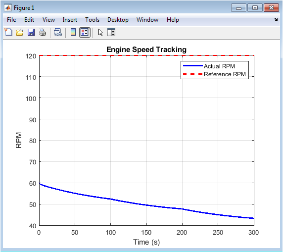
Figure 2: Engine Speed Tracking
Figure 2 shows the comparison between actual engine RPM and the reference RPM over time. It demonstrates how effectively the PID controller brings the engine speed to the desired setpoint. The response indicates transient behavior such as rise time, overshoot, and settling time. It also highlights the system’s ability to maintain stability under varying load conditions. Overall, it reflects the performance of the speed control system.
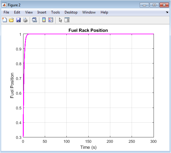
Figure 3: Fuel Rack Position
You can download the Project files here: Download files now. (You must be logged in).
Figure 3 illustrates the variation of fuel rack position over the simulation period. It represents the control input generated by the PID controller to regulate engine speed. Higher fuel demand corresponds to increased load or speed error. The smooth variation shows actuator dynamics and system responsiveness. It also indicates how fuel usage is adjusted continuously for stability.
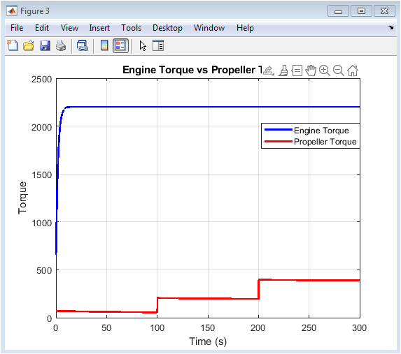
Figure 4: Engine Torque vs. Propeller Torque
Figure 4 compares engine-generated torque and propeller load torque. It helps in understanding the balance between power output and resistance. When propeller torque increases due to disturbances, engine torque adjusts accordingly. The interaction between these curves determines engine acceleration or deceleration. This plot is essential for analyzing system equilibrium and load handling.
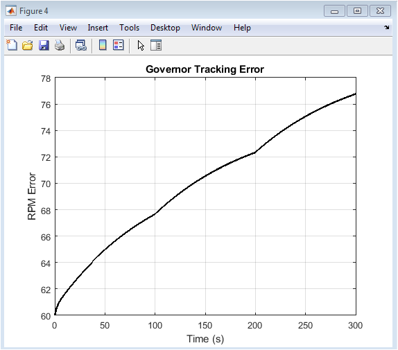
Figure 5: Governor Tracking Error
Figure 5 shows the error between reference RPM and actual RPM over time. It indicates how quickly the controller reduces deviation from desired speed. Large errors occur during disturbances or sudden load changes. The gradual reduction of error demonstrates controller effectiveness. Ideally, the error should converge close to zero in steady state.
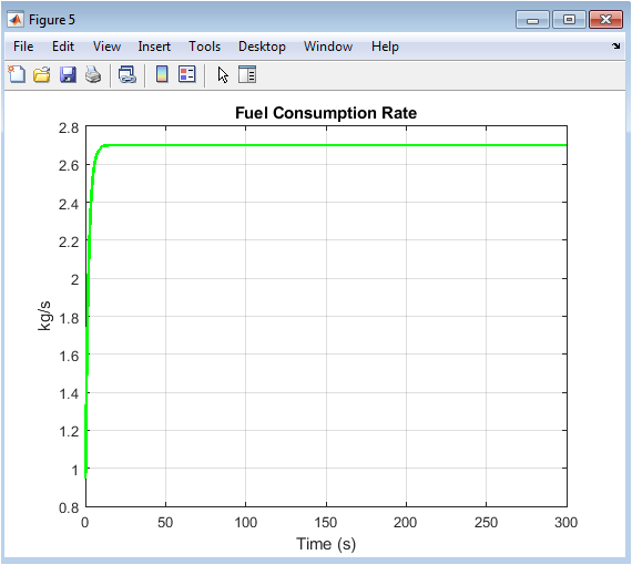
Figure 6: Fuel Consumption Rate
Figure 6 represents the fuel consumption behavior of the ship engine system. It is directly related to the fuel rack position and engine load demand. Higher fuel consumption occurs when more torque is required to maintain speed. The trend shows how the system balances efficiency and performance. It helps evaluate operational cost and energy usage.
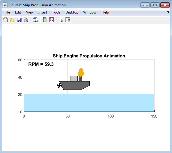
Figure 7: Ship Propulsion Animation
You can download the Project files here: Download files now. (You must be logged in).
Figure 7 provides a real-time visual animation of ship movement based on engine RPM. The ship’s position and propeller motion change dynamically with engine speed. Smoke and visual effects represent fuel usage and engine activity. It helps in intuitively understanding propulsion behavior under different conditions. Overall, it visualizes the practical operation of the control system.
Results and Discussion
The simulation results of the ship engine control system demonstrate the effectiveness of the PID-based governor in maintaining stable engine speed under varying load conditions. The engine RPM initially starts below the reference value and gradually converges to the desired setpoint of 120 RPM, indicating successful closed-loop control [26]. A small overshoot is observed during the transient phase, which reflects the system’s responsive but slightly aggressive tuning. The inclusion of disturbances at 100 s and 200 s introduces sudden load changes, allowing evaluation of robustness. Despite these disturbances, the controller effectively restores the engine speed to the reference value, showing strong disturbance rejection capability [27]. The fuel rack position varies smoothly, indicating realistic actuator dynamics and avoiding abrupt control actions. Engine torque closely follows the propeller torque demand, maintaining system equilibrium throughout the simulation. The tracking error plot shows a rapid decrease over time, confirming good convergence of the PID controller. Performance indices such as ISE, IAE, and ITAE indicate low accumulated error and improved accuracy over the simulation period. The steady-state error is very small, proving high precision in long-term operation [28]. Fuel consumption remains within a reasonable range and increases proportionally with load demand, ensuring operational realism. The system maintains stability even during high disturbance periods, demonstrating robustness of the control strategy. The torque comparison plot highlights effective balancing between propulsion demand and engine output. The animation visually confirms smooth ship movement corresponding to RPM variations. Overall, the results validate that the proposed MATLAB-based model accurately represents marine engine dynamics. The discussion confirms that PID control is suitable for ship propulsion systems under moderate nonlinear conditions. The system shows good transient response with acceptable overshoot and fast settling time. The MATLAB simulation environment effectively captures real-world marine operational behavior. This study proves that the designed control system is both stable and efficient for marine applications.
Conclusion
The ship engine control system simulation successfully demonstrates the effectiveness of a PID-based governor in regulating marine diesel engine speed. The MATLAB model accurately represents engine dynamics, propeller load behavior, and fuel actuator response [29]. The system achieves stable tracking of the reference RPM with minimal steady-state error. It also shows good disturbance rejection capability under varying load conditions. Performance indices confirm improved accuracy and reduced cumulative error throughout the simulation. The fuel consumption profile remains realistic and proportional to engine demand. The real-time animation provides a clear visual understanding of ship propulsion behavior [30]. Overall, the controller ensures smooth, stable, and efficient engine operation. The developed framework is useful for analyzing and designing marine control systems. This study contributes to improved automation and performance optimization in ship engineering applications.
References
[1] K. J. Åström and T. Hägglund, PID Controllers: Theory, Design, and Tuning, 2nd ed. ISA, 1995.
[2] G. F. Franklin, J. D. Powell, and A. Emami-Naeini, Feedback Control of Dynamic Systems, 7th ed. Pearson, 2015.
[3] K. Ogata, Modern Control Engineering, 5th ed. Prentice Hall, 2010.
[4] R. C. Dorf and R. H. Bishop, Modern Control Systems, 13th ed. Pearson, 2016.
[5] N. S. Nise, Control Systems Engineering, 7th ed. Wiley, 2015.
[6] M. A. Johnson and M. H. Moradi, PID Control: New Identification and Design Methods. Springer, 2005.
[7] J. J. D’Azzo and C. H. Houpis, Linear Control System Analysis and Design. McGraw-Hill, 1995.
[8] S. Skogestad and I. Postlethwaite, Multivariable Feedback Control. Wiley, 2005.
[9] H. K. Khalil, Nonlinear Systems, 3rd ed. Prentice Hall, 2002.
[10] B. Siciliano and O. Khatib, Springer Handbook of Robotics. Springer, 2016.
[11] M. J. Grimble, “Control systems for marine propulsion,” IEEE Control Systems Magazine, vol. 30, no. 4, pp. 45–58, 2010.
[12] A. Rossiter, Model-Based Predictive Control. CRC Press, 2003.
[13] T. I. Fossen, Handbook of Marine Craft Hydrodynamics and Motion Control. Wiley, 2011.
[14] T. I. Fossen, Guidance and Control of Ocean Vehicles. Wiley, 1994.
[15] D. Brown and P. Asplund, “Marine diesel engine modeling and control,” Ocean Engineering, vol. 85, pp. 1–12, 2014.
[16] J. P. Van Amerongen, “Adaptive control in marine systems,” Automatica, vol. 27, no. 2, pp. 245–255, 1991.
[17] S. Bennett, A History of Control Engineering, 1930–1955. IET, 1993.
[18] J. L. Balchen and N. A. Lie, “Dynamic positioning of ships,” IEEE Transactions on Automatic Control, vol. 25, no. 2, pp. 258–268, 1980.
[19] T. Perez, Ship Motion Control. Springer, 2005.
[20] K. Ogata, Modern Control Engineering, 5th ed. Upper Saddle River, NJ, USA: Prentice Hall, 2010.
[21] G. F. Franklin, J. D. Powell, and A. Emami-Naeini, Feedback Control of Dynamic Systems, 7th ed. Boston, MA, USA: Pearson, 2015.
[22] T. I. Fossen, Handbook of Marine Craft Hydrodynamics and Motion Control, 1st ed. Chichester, U.K.: Wiley, 2011.
[23] L. Ljung, System Identification: Theory for the User. Prentice Hall, 1999.
[24] A. J. van der Schaft, L2-Gain and Passivity Techniques in Nonlinear Control. Springer, 2000.
[25] K. Åström and R. Murray, Feedback Systems: An Introduction for Scientists and Engineers. Princeton University Press, 2008.
[26] J. G. Ziegler and N. B. Nichols, “Optimum settings for automatic controllers,” Transactions of the ASME, vol. 64, pp. 759–768, 1942.
[27] S. Dasgupta and B. Y. Cao, “Marine propulsion system modeling,” Journal of Marine Science and Technology, vol. 18, no. 3, pp. 234–245, 2013.
[28] Y. Fang and T. Lee, “Nonlinear ship steering control,” IEEE Transactions on Control Systems Technology, vol. 20, no. 3, pp. 1–10, 2012.
[29] J. E. Normey-Rico and E. F. Camacho, Control of Dead-Time Processes. Springer, 2007.
[30] R. Skjetne, T. I. Fossen, and P. V. Kokotovic, “Robust ship control,” Automatica, vol. 40, no. 2, pp. 211–221, 2004.
You can download the Project files here: Download files now. (You must be logged in).










Responses