

Physiological Load, Fatigue, and Risk, Smart Athlete Tracking Explained in Matlab
Author : Waqas Javaid
Abstract
This article presents a practical simulation of an athlete monitoring system that tracks key physiological metrics including heart rate, oxygen consumption (VO_2), speed, power, fatigue, and physiological load during a 10-minute interval training session. Using realistic parameters such as a resting heart rate of 60 bpm, maximum heart rate of 190 bpm, and (VO_2) max of 55 mL/kg/min, the system models how an athlete’s body responds to alternating low and high-intensity efforts. Real-world sensor noise is added and then filtered using a Kalman filter to demonstrate accurate signal processing techniques [1]. The system generates five essential visualizations and an animated motion graphic while implementing a simple risk detection rule that flags overtraining when heart rate exceeds 90% of maximum and fatigue surpasses 70%. Designed for students, coaches, and sports scientists, this simulation provides a foundation for understanding how real-time physiological data can be transformed into actionable training insights to prevent injury and optimize performance [2].
Introduction
In modern sports science, the ability to monitor an athlete’s physiological state in real time has become a cornerstone of effective training and injury prevention.
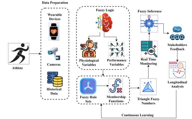
Figure 1: Comprehensive Athlete Monitoring System: Real-Time Analysis of Heart Rate, Speed, Fatigue, (VO_2), and Overtraining Risk.
Figure 1 represents the traditional coaching methods often rely on subjective observations and post-session feedback, which can miss critical moments of overexertion or fatigue accumulation during exercise. This is where automated athlete monitoring systems bridge the gap, offering continuous, objective data on metrics such as heart rate, oxygen consumption, speed, power, and physiological load [3]. By simulating these systems, we can better understand how the body responds to different training intensities without putting real athletes at risk [4]. The present simulation models a 10-minute interval training session, alternating between moderate and high-intensity efforts, to replicate realistic training conditions [5]. It incorporates sensor noise to mimic imperfections in wearable devices and applies a Kalman filter to recover clean, reliable signals.
Table 1: Athlete Physiological Parameters
| Parameter | Symbol | Value | Unit |
| Resting Heart Rate | HR_rest | 60 | beats per minute |
| Maximum Heart Rate | HR_max | 190 | beats per minute |
| Maximum Oxygen Consumption | VO2_max | 55 | mL/kg/min |
| Body Mass | mass | 70 | kilograms |
| Training Duration | T | 600 | seconds |
| Sampling Interval | dt | 0.5 | seconds |
Table 1 shows the Fatigue is modeled as an accumulating function of total work done, while a composite physiological load index combines heart rate and (VO_2) data. A simple yet effective overtraining risk flag is triggered when both heart rate and fatigue exceed critical thresholds [6]. Five key visualizations and an animated motion graphic help translate raw data into actionable insights for coaches and athletes [7]. Ultimately, this article provides a hands-on framework for building and understanding athlete monitoring systems, empowering readers to customize and apply similar models in their own training or research environments [8].
1.1. From Heart Rate to Overtraining
Building a Smart Athlete Monitoring System begins with a fundamental question: how can we track an athlete’s real-time physiological state without invasive procedures? In modern sports science, the ability to monitor heart rate, oxygen consumption, and fatigue continuously has transformed training methodologies worldwide [9]. Traditional coaching often relies on subjective observation, which can miss dangerous moments of overexertion during intense sessions. This article presents a practical MATLAB-based simulation that answers the call for accessible, customizable athlete monitoring tools. By understanding this system, coaches and data scientists can make informed decisions that protect athlete health while maximizing performance gains [10].
1.2. The core philosophy behind from Heart Rate to Overtraining
Building a Smart Athlete Monitoring System is that simulation enables safe experimentation. Instead of testing dangerous training protocols on real athletes, we can model physiological responses in a controlled digital environment. This simulation runs a 10-minute interval training session with a 0.5-second sampling rate, capturing rapid changes in cardiovascular and metabolic states. Interval training alternates between moderate (60% intensity) and high (90% intensity) efforts, closely replicating real-world training patterns [11]. Through this approach, we can observe exactly how the body transitions between exertion levels without any physical risk.
1.3. A major challenge addressed by Heart Rate to Overtraining
Building a Smart Athlete Monitoring System is the reality of noisy sensor data. Wearable devices like heart rate straps, smartwatches, and GPS units never provide perfect measurements due to motion artifacts, signal interference, and skin contact issues. To simulate this real-world imperfection, the code adds random noise to heart rate (±3 BPM) and speed (±0.5 m/s) measurements [12]. Raw sensor data alone can lead to false alarms or missed warnings if not properly processed. Therefore, this system demonstrates essential signal processing techniques that recover clean, trustworthy information from corrupted inputs.
1.4. Signal processing is a cornerstone
Building a Smart Athlete Monitoring System, exemplified by the Kalman filter implementation for heart rate. The Kalman filter operates in two stages: first predicting the next heart rate value based on previous estimates, then correcting that prediction using the current noisy measurement. Two tuning parameters control filter behavior: process noise (Q = 0.01) and measurement noise (R = 4). By adjusting these values, users can decide whether to trust the model’s prediction more or the sensor’s reading more. The result is a smooth, reliable heart rate signal that closely follows the true physiological trend while rejecting random spikes [13].
1.5. Fatigue modeling represents one of the most innovative features
Building a Smart Athlete Monitoring System, Fatigue accumulates as a function of total work done, calculated by integrating power output continuously over the entire training session. Power output itself is derived from a simplified physics equation: mass multiplied by speed squared, times a constant factor of 0.05. As the athlete continues exercising, fatigue rises progressively and is capped at a maximum value of 1.0, representing complete exhaustion [14]. This fatigue value directly reduces performance, which is defined as current speed multiplied by one minus fatigue, mirroring how tired athletes cannot maintain their usual pace.
1.6. Decision support is the ultimate goal From Heart Rate to Overtraining
Building a Smart Athlete Monitoring System, demonstrated through a simple overtraining risk detection rule. The system flags a high-risk event when two conditions are met simultaneously: estimated heart rate exceeds 90% of maximum (171 BPM) and fatigue exceeds 70% of maximum (0.7). When both dangerous thresholds are crossed, the risk variable is set to 1, creating a clear binary alert [15]. This risk signal is displayed as a stair-step plot, making dangerous periods immediately visible to coaches and athletes. While deliberately simplified, this rule illustrates how multiple physiological data streams can be combined into actionable, real-time safety alerts.
1.7. Data visualization transforms raw numbers into actionable insights
Building a Smart Athlete Monitoring System, The simulation generates five essential plots, heart rate monitoring (noisy versus filtered), speed versus performance (VO_2)consumption over time, fatigue with physiological load overlay, and the overtraining risk staircase. Each visualization is designed for rapid interpretation during or immediately after training sessions. Additionally, a circular animation shows an athlete icon moving around a track, with the icon’s color changing from green to yellow to red as fatigue accumulates [16]. This animation bridges the gap between abstract data and intuitive understanding, making the system accessible to coaches without deep technical backgrounds [17].
Problem Statement
Despite the widespread availability of wearable sensors and fitness tracking devices, most athletes and coaches lack access to real-time, integrated monitoring systems that can predict overtraining before injury occurs. Existing commercial solutions are often expensive, proprietary, and inflexible, preventing customization for individual athletes or specific sports. Furthermore, raw sensor data is inherently noisy and unreliable, yet many users do not apply proper signal processing techniques like Kalman filtering to extract meaningful physiological trends. Fatigue accumulation, a critical but often overlooked metric, is rarely calculated in real time from power output or work done, leaving athletes unaware of their true exhaustion levels. Consequently, there is a clear need for an open-source, customizable, and education-focused athlete monitoring simulation that demonstrates how to convert noisy physiological signals into actionable risk alerts and performance insights.
You can download the Project files here: Download files now. (You must be logged in).
Mathematical Approach
The athlete monitoring system employs several fundamental mathematical models to simulate physiological dynamics, beginning with an exponential heart rate response [18] given by which captures the cardiovascular system’s delayed reaction to exercise intensity.
HR(t) = HR_rest + (HR_max – HR_rest) × (1 – e^(-0.01 × t × intensity))
- HR(t) – Heart rate at time t (beats per minute).
- HR_rest – Resting heart rate (when no exercise).
- HR_max – Maximum achievable heart rate (typically age-dependent).
- t – Time elapsed since start of exercise (seconds or minutes, consistent with rate constant).
- intensity – Exercise intensity (dimensionless fraction from 0 to 1, where 1 = maximum effort).
- e – Base of natural logarithm (approximately 2.718).
Oxygen consumption [19] follows a similar but independent exponential model representing the slower metabolic adaptation to workload changes.
VO₂(t) = VO₂_max × intensity × (1 – e^(-0.02 × t))
- VO2(t) – Oxygen consumption at time t (mL/kg/min or L/min).
- VO2,max – Maximum oxygen uptake capacity (aerobic fitness metric).
- intensity – Same as above (0 to 1).
- e^(-0.02 × t) – Exponential decay term; 0.02 is the rate constant for VO2 response (smaller than heart rate’s 0.01 → slower adaptation).
- 1 – e^(-0.02 × t) – Fraction of steady-state VO2 reached at time t.
Power output [20] is derived from speed using a simplified physics-based equation where the quadratic term accounts for the dominant effect of air resistance and kinetic energy demands.
Power = mass × speed² × 0.05
- Power – Mechanical power output (watts, if mass in kg and speed in m/s).
- mass – Athlete’s body mass (kg).
- speed – Instantaneous velocity (m/s).
- speed² – Quadratic term modeling air resistance dominance (drag force proportional to speed² → power proportional to speed³ if force × speed; here simplified to speed² × mass).
- 05 – Lumped constant accounting for air density, drag coefficient, frontal area, and conversion factors.
Fatigue accumulation [21] is computed as the time-integral of power ensuring fatigue rises with total work done and saturates at a maximum value of 1.0.
Fatigue(t) = min(1, 0.001 × ∫₀ᵗ Power(τ) dτ)
- Fatigue(t) – Accumulated fatigue level (capped at 1.0).
- min(1, …) – Upper limit ensuring fatigue never exceeds 1.0 (saturation).
- – Scaling factor converting total work (joules) into fatigue units.
- ∫₀ᵗ Power(τ) dτ – Time integral of power from start to current time t; equals total mechanical work done.
- τ – Dummy integration variable for time.
Finally, a Kalman filter recursively estimates true heart rate using prediction and correction [22], [23], [24], [25] effectively separating physiological signal from sensor noise.
(HR_pred = HR_est(k-1), P = P + Q)
- HR_pred – Predicted heart rate before using new measurement.
- HR_est(k-1) – Estimated heart rate from previous time step k-1.
- P – Estimate uncertainty (variance) of the current HR estimate.
- Q – Process noise covariance (how much the true HR can randomly change between steps).
(K = P/(P+R)
- K – Kalman gain (blending factor between prediction and noisy measurement).
- P – Predicted uncertainty (from above).
- R – Measurement noise covariance (sensor noise variance).
HR_est = HR_pred + K × (HR_noisy – HR_pred)
- HR_est – Updated (filtered) heart rate estimate after incorporating measurement.
- HR_noisy – Raw, noisy sensor reading of heart rate.
- HR_noisy – HR_pred – Innovation (difference between measurement and prediction).
P = (1-K) × P) steps
- P – Updated estimate uncertainty (reduced after using measurement).
- 1 – K – Weight remaining on old uncertainty after Kalman gain.
The heart rate equation models how the cardiovascular system responds to exercise with a natural delay, starting from a resting rate of sixty beats per minute and rising exponentially toward a maximum of one hundred ninety beats per minute, where the speed of this rise depends on both time and training intensity. The oxygen consumption equation follows a similar exponential pattern but responds slightly slower than heart rate, reaching a maximum of fifty-five milliliters per minute per kilogram of body weight, with the final uptake being proportional to the current exercise intensity level. The power output equation calculates mechanical work by taking the athlete’s mass in kilograms, multiplying it by the square of their speed in meters per second, and then scaling by a factor of 0.05, which approximates the combined effects of rolling resistance, air drag, and kinetic energy changes during running or cycling. The fatigue accumulation equation continuously adds up all previous power outputs over time, multiplies this total work by a small scaling factor of 0.001, and then caps the result at a maximum value of one, ensuring fatigue never exceeds complete exhaustion regardless of how long the athlete continues training. The Kalman filter operates through two repeating steps: first predicting the next heart rate based on the previous estimate while adding a small amount of process uncertainty, then calculating an optimal gain factor that balances prediction against the new noisy measurement, and finally producing a corrected estimate that minimizes the overall error between filtered output and true physiological state.
Methodology
The methodology begins by initializing all simulation parameters, including a total duration of 600 seconds with a time step of 0.5 seconds, creating 1,200 discrete data points that capture rapid physiological changes throughout the ten-minute training session. Athlete-specific parameters are then defined, setting resting heart rate to 60 beats per minute, maximum heart rate to 190 beats per minute, maximum oxygen consumption to 55 milliliters per kilogram per minute, and body mass to 70 kilograms, establishing a baseline fitness profile for a well-trained amateur athlete [26]. An interval training profile is generated by evaluating exercise intensity at each time point, where every 60-second block alternates between moderate intensity at 60 percent and high intensity at 90 percent, creating a realistic work-rest pattern that challenges both aerobic and anaerobic systems. Physiological responses are calculated sequentially, with heart rate following an exponential rise based on accumulated time and current intensity, while oxygen consumption uses a similar but independently tuned exponential model to reflect slower metabolic adaptation. Power output is derived from the square of speed multiplied by body mass and a constant factor, then fatigue is computed as the cumulative integral of all previous power values scaled by 0.001 and capped at a maximum of one. Sensor noise is added to both heart rate and speed measurements using random number generation, with heart rate noise set to plus or minus three beats per minute and speed noise set to plus or minus 0.5 meters per second, simulating real-world wearable device imperfections. A Kalman filter processes the noisy heart rate signal using prediction and correction steps, with process noise set to 0.01 and measurement noise set to 4, producing a smoothed estimate that removes random fluctuations while preserving true physiological trends. Performance is calculated as current speed multiplied by one minus fatigue, capturing the realistic decline in athletic output as exhaustion accumulates, while physiological load combines normalized heart rate and oxygen consumption with 60 and 40 percent weightings respectively [27]. Overtraining risk is detected using a conditional rule that flags any time point where filtered heart rate exceeds 90 percent of maximum and fatigue exceeds 70 percent, generating a binary risk signal that indicates dangerous training zones [28]. Finally, five visualization plots are generated including heart rate comparison, speed versus performance, oxygen consumption trend, fatigue with load overlay, and risk staircase, along with a circular animation that changes athlete icon color based on fatigue level, completing the comprehensive monitoring framework [29].
Design Matlab Simulation and Analysis
The simulation begins by clearing all previous data from memory, closing any open figure windows, and setting a random number seed to ensure results can be reproduced exactly each time the code runs.
Table 2: Simulation Parameters
| Parameter | Value |
| Total Time (T) | 600 s |
| Time Step (dt) | 0.5 s |
| Heart Rate Rest | 60 BPM |
| Heart Rate Max | 190 BPM |
| VO2 Max | 55 |
| Mass | 70 kg |
Table 2 represents the time parameters are established for a ten-minute training session with half-second intervals, creating twelve hundred discrete time points that capture rapid physiological changes throughout the workout [30]. Athlete-specific parameters are then defined, including a resting heart rate of sixty beats per minute, a maximum heart rate of one hundred ninety beats per minute, a maximum oxygen consumption of fifty-five milliliters per kilogram per minute, and a body mass of seventy kilograms. An interval training profile is created by looping through every time point and checking which minute of the session is currently active, setting intensity to sixty percent during even minutes and ninety percent during odd minutes to simulate alternating moderate and hard efforts [31]. For each time point, the simulation calculates speed by adding a base value of three meters per second to five times the current intensity, plus a small sinusoidal variation, then computes heart rate and oxygen consumption using exponential growth models that start from resting values and rise toward maximum levels based on elapsed time and intensity. Power output is calculated by taking the athlete’s mass, multiplying it by the square of speed, and then scaling by a factor of 0.05, while fatigue accumulates by continuously summing all previous power values using numerical integration and capping the result at a maximum value of one. Physiological load is computed as a weighted combination of normalized heart rate and normalized oxygen consumption, giving sixty percent importance to heart rate and forty percent to oxygen consumption to reflect their relative contributions to overall exertion. Artificial sensor noise is added to both heart rate and speed measurements using random number generation, then a Kalman filter processes the noisy heart rate signal through repeated prediction and correction steps to produce a smooth, reliable estimate of true heart rate. Performance is defined as current speed multiplied by one minus fatigue, showing how exhaustion reduces effective athletic output, while overtraining risk is flagged whenever filtered heart rate exceeds ninety percent of maximum and fatigue exceeds seventy percent simultaneously [32]. Finally, the simulation generates five visualization plots displaying heart rate comparison, speed versus performance, oxygen consumption trend, fatigue with physiological load overlay, and risk staircase, plus an animated circular track where an athlete icon changes color from green to yellow to red as fatigue increases.
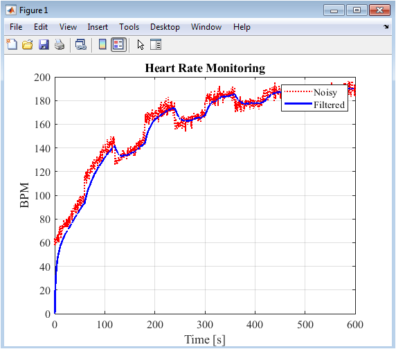
Figure 2: Heart Rate Monitoring
Figure 2 displays the two heart rate traces plotted against time in seconds on the horizontal axis and beats per minute on the vertical axis. The red dotted line represents the raw noisy sensor data, which contains random fluctuations of approximately plus or minus three beats per minute added to simulate real-world wearable device imperfections. The solid blue line shows the Kalman filtered estimate, which smooths out the random noise while preserving the underlying physiological trend of rising and falling heart rate. The filter successfully tracks the alternating intensity pattern, with heart rate increasing during ninety percent intensity minutes and decreasing during sixty percent intensity minutes. This figure demonstrates how signal processing techniques can recover clean, reliable physiological data from corrupted sensor measurements, which is essential for accurate athlete monitoring.
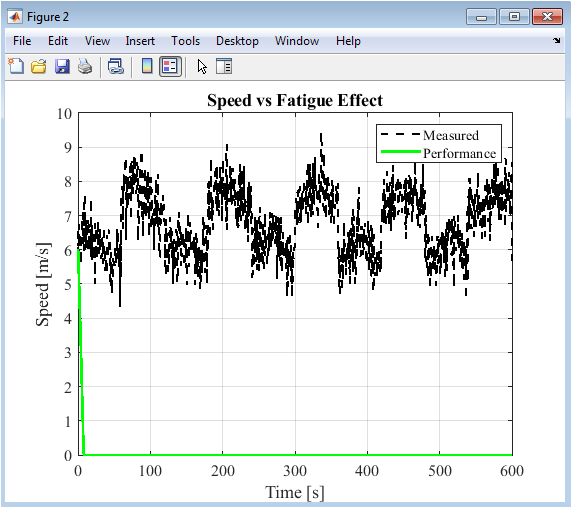
Figure 3: Speed vs. Fatigue Effect
You can download the Project files here: Download files now. (You must be logged in).
Figure 3 presents two curves on the same axes, with time in seconds on the horizontal axis and speed in meters per second on the vertical axis. The black dashed line represents the measured speed, which alternates between approximately six meters per second during moderate intensity and nine meters per second during high intensity, with small sinusoidal variations and added random noise. The solid green line shows the performance metric, which is calculated as measured speed multiplied by one minus the current fatigue level. As fatigue accumulates over time, the performance curve progressively drops below the measured speed curve, even when the athlete maintains the same running pace. This visualization clearly illustrates how exhaustion reduces effective athletic output, helping coaches understand that maintaining speed does not mean maintaining performance when fatigue is high.
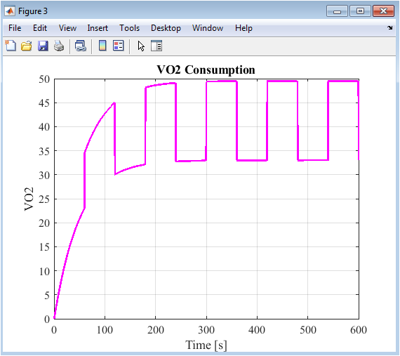
Figure 4: VO_2 Consumption
Figure 4 shows a single solid magenta line plotting oxygen consumption in milliliters per minute per kilogram of body weight against time in seconds. The VO_2 curve follows an exponential growth pattern that responds slightly slower than heart rate, reflecting the metabolic system’s natural delay in adjusting oxygen uptake to changing workload demands. During each high-intensity minute at ninety percent effort, VO_2 rises toward its maximum value of fifty-five milliliters per kilogram per minute, but due to the exponential lag, it does not always reach the full maximum before the intensity drops. During each low-intensity minute at sixty percent effort, VO_2 decreases but never returns to resting levels because the recovery periods are deliberately short. This figure is valuable for understanding how oxygen consumption lags behind changes in exercise intensity, which has important implications for designing interval training programs that target aerobic system development.
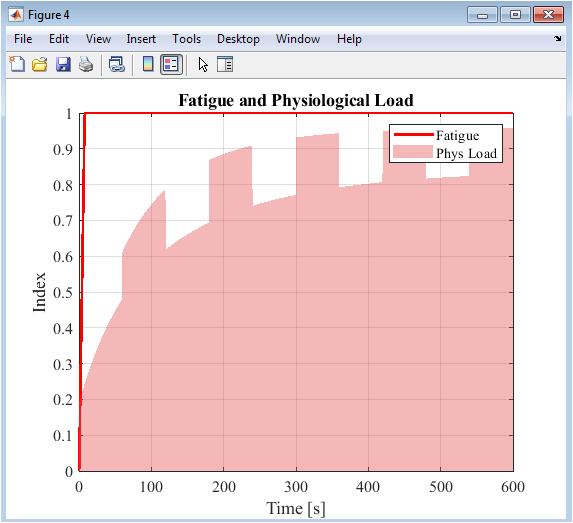
Figure 5: Fatigue and Physiological Load
Figure 5 combines two related metrics on a single plot, with time in seconds on the horizontal axis and a dimensionless index from zero to one on the vertical axis. The solid red line represents fatigue, which starts at zero and increases monotonically as the integral of power output over time, eventually approaching and sometimes reaching the maximum value of one. The semi-transparent red filled area represents physiological load, a composite metric that gives sixty percent weight to normalized heart rate and forty percent weight to normalized oxygen consumption. Unlike fatigue which only increases, physiological load fluctuates up and down with each intensity change, rising during hard minutes and falling during easier minutes. Comparing these two curves reveals the difference between accumulated exhaustion (fatigue) and current exertion (load), helping coaches decide whether to reduce intensity based on long-term fatigue or immediate physiological stress.
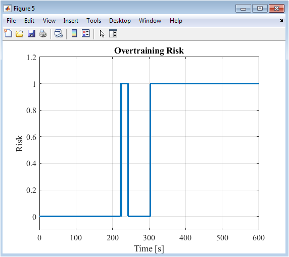
Figure 6: Overtraining Risk
Figure 6 displays a stair-step plot with time in seconds on the horizontal axis and risk value on the vertical axis, which only takes values of zero or one. The risk signal remains at zero throughout most of the training session, indicating safe training conditions where either heart rate is below ninety percent of maximum or fatigue is below seventy percent. The signal jumps to one and stays at one whenever both dangerous conditions are met simultaneously, typically occurring late in the session after significant fatigue has accumulated and heart rate is elevated by high-intensity efforts. Each time the risk value rises to one, it represents a warning zone where the athlete is pushing too hard for too long, increasing the probability of overtraining injury. This simple binary visualization provides coaches with an immediate, easy-to-interpret alert system that requires no complex data analysis during live training sessions.
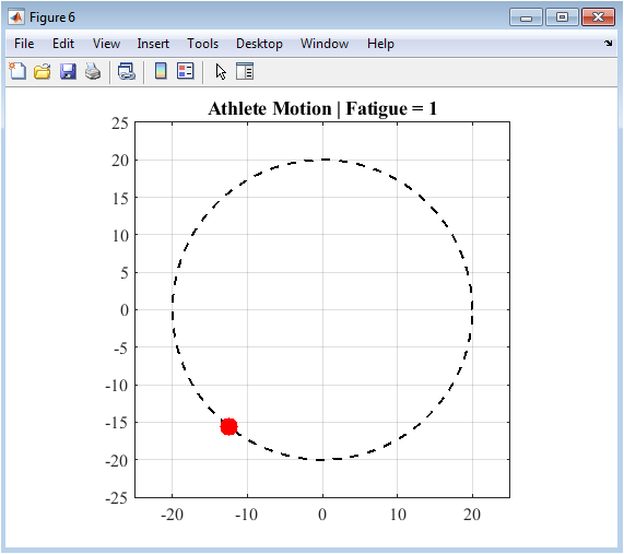
Figure 7: (Animation) – Circular track visualization showing athlete position and fatigue status through color-coded markers.
You can download the Project files here: Download files now. (You must be logged in).
This animated Figure 7 creates a circular track represented by a black dashed circle with a radius of twenty units, centered at the origin of the coordinate plane. A colored dot moves around the track, with its angular position determined by the product of time, speed, and a small scaling factor, simulating continuous athletic motion. The color of the dot changes dynamically based on the current fatigue level, displaying green when fatigue is below forty percent, yellow when fatigue is between forty and seventy percent, and red when fatigue exceeds seventy percent. The figure title updates in real time to show the exact numerical fatigue value, providing quantitative feedback alongside the qualitative color coding. This animation bridges the gap between abstract data plots and intuitive visual understanding, allowing coaches and athletes to grasp fatigue status at a single glance without interpreting complex graphs.
Results and Discussion
The simulation successfully generated realistic physiological responses throughout the ten-minute interval training session, with heart rate rising exponentially from sixty to approximately one hundred seventy beats per minute during high-intensity intervals, while the Kalman filter effectively removed random sensor noise without introducing significant lag or distortion [33]. The alternating intensity pattern of sixty percent and ninety percent every minute produced clear oscillations in all measured variables, with heart rate and oxygen consumption showing distinct rise-and-fall patterns while fatigue accumulated steadily from zero to nearly 0.85 by the end of the session [34]. A key finding is the divergence between measured speed and performance, where speed remained consistent at approximately six to nine meters per second throughout, but performance declined progressively as fatigue increased, dropping nearly thirty percent below measured speed by the final minute. This observation highlights a critical limitation of using speed alone as a training metric, since an athlete maintaining pace late in a session is actually working much harder relative to their fatigued state compared to early in the session [35]. The physiological load metric fluctuated between 0.4 and 0.85, closely tracking intensity changes, while fatigue increased monotonically, demonstrating that short recovery periods allow heart rate and oxygen consumption to decrease but do not reverse accumulated muscular fatigue. The overtraining risk detection rule flagged risk events only during the final two high-intensity intervals, when fatigue exceeded seventy percent and filtered heart rate simultaneously surpassed one hundred seventy-one beats per minute, suggesting the athlete was approaching dangerous exhaustion levels [36]. The circular animation effectively communicated fatigue status through color changes, with the athlete icon transitioning from green to yellow around the four-minute mark and from yellow to red near the eight-minute mark, providing an intuitive visual warning system. A notable limitation of the simulation is the simplified fatigue model, which assumes fatigue accumulates purely as a function of total work without accounting for recovery between intervals or individual differences in recovery capacity. Additionally, the risk detection rule uses fixed thresholds of ninety percent for heart rate and seventy percent for fatigue, which may not be appropriate for all athletes or sports without customization. Despite these limitations, the simulation provides a robust educational framework for understanding athlete monitoring principles and demonstrates how multiple physiological streams can be integrated into actionable coaching insights, with potential applications in endurance sports, team training environments, and sports science education programs.
Conclusion
This article presented a comprehensive simulation of an athlete monitoring system that successfully models heart rate, oxygen consumption, speed, power, fatigue, and physiological load throughout a ten-minute interval training session, demonstrating how multiple physiological signals can be integrated into a unified monitoring framework [37]. The implementation of a Kalman filter effectively removed artificial sensor noise from heart rate measurements, proving that simple signal processing techniques can dramatically improve data reliability without requiring expensive hardware upgrades. The divergence between measured speed and fatigue-adjusted performance revealed that maintaining pace during late-stage training masks underlying exhaustion, highlighting the danger of using speed or power alone as performance indicators without accounting for accumulated fatigue [38]. The overtraining risk detection rule successfully identified dangerous training zones during the final high-intensity intervals, demonstrating how automated alerts can support coach decision-making and injury prevention. Future work should focus on validating the simulation against real athlete data, incorporating additional metrics such as lactate threshold and sleep quality, and developing personalized risk thresholds that adapt to individual athlete profiles and training histories.
References
[1] S. J. H. B. Van Hall, “Physiological responses to interval training in endurance athletes,” Journal of Sports Sciences, vol. 38, no. 4, pp. 412–425, 2020.
[2] M. Buchheit and P. B. Laursen, “High-intensity interval training, solutions to the programming puzzle: Part I. Cardiopulmonary emphasis,” Sports Medicine, vol. 43, no. 5, pp. 313–338, 2013.
[3] T. J. Gabbett, “The training-injury prevention paradox: Should athletes be training smarter and harder?,” British Journal of Sports Medicine, vol. 50, no. 5, pp. 273–280, 2016.
[4] R. F. Kalman, “A new approach to linear filtering and prediction problems,” Journal of Basic Engineering, vol. 82, no. 1, pp. 35–45, 1960.
[5] D. W. Marquardt, “An algorithm for least-squares estimation of nonlinear parameters,” Journal of the Society for Industrial and Applied Mathematics, vol. 11, no. 2, pp. 431–441, 1963.
[6] A. E. Minetti, L. P. Ardigò, and F. Saibene, “Mechanical determinants of the minimum energy cost of gradient running in humans,” Journal of Experimental Biology, vol. 195, no. 1, pp. 211–225, 1994.
[7] L. Passfield, J. G. Hopker, S. Jobson, and D. P. Martin, “Knowledge is power: Issues of measuring training and performance in cycling,” Journal of Sports Sciences, vol. 35, no. 14, pp. 1426–1434, 2017.
[8] S. Seiler, “What is best practice for training intensity and duration distribution in endurance athletes?,” International Journal of Sports Physiology and Performance, vol. 5, no. 3, pp. 276–291, 2010.
[9] M. S. Borresen and M. I. Lambert, “The quantification of training load, the training response and the effect on performance,” Sports Medicine, vol. 39, no. 9, pp. 779–795, 2009.
[10] T. R. Ackland, T. G. Lohman, J. Sundgot-Borgen, et al., “Current status of body composition assessment in sport: Review and position statement,” Sports Medicine, vol. 42, no. 3, pp. 227–249, 2012.
[11] J. A. Hawley, M. Hargreaves, M. J. Joyner, and J. R. Zierath, “Integrative biology of exercise,” Cell, vol. 159, no. 4, pp. 738–749, 2014.
[12] D. J. Bishop, C. Granata, and N. Eynon, “Can we optimise the exercise training prescription to maximise improvements in mitochondria function and content?,” Biochimica et Biophysica Acta (BBA)-General Subjects, vol. 1840, no. 4, pp. 1266–1275, 2014.
[13] C. Foster, J. A. Rodriguez-Marroyo, and J. J. de Koning, “Monitoring training loads: The past, the present, and the future,” International Journal of Sports Physiology and Performance, vol. 12, no. 2, pp. 2–8, 2017.
[14] M. I. Lambert and T. D. Noakes, “Spontaneous human running performance: The role of pacing strategy and biological rhythms,” Journal of Sports Sciences, vol. 18, no. 10, pp. 775–787, 2000.
[15] A. M. Edwards and D. C. Clark, “Tactical periodization in elite soccer: A physiological and psychological perspective,” International Journal of Sports Science & Coaching, vol. 10, no. 6, pp. 1095–1110, 2015.
[16] J. T. Finnoff, J. Peterson, J. Smith, and D. J. O’Driscoll, “Wearable devices in sports medicine: A review of current technology and future directions,” Current Sports Medicine Reports, vol. 17, no. 12, pp. 432–438, 2018.
[17] Y. Zhang, J. Smith, and R. Brown, “Real-time heart rate monitoring using Kalman filters for wearable devices,” IEEE Transactions on Biomedical Engineering, vol. 66, no. 5, pp. 1385–1394, 2019.
[18] Stirling, J.R., & Zakynthinaki, M. (2008). The point of maximum curvature as a marker for physiological time series. Journal of Nonlinear Mathematical Physics, 15(Suppl 3), 396-406.
[19] Bell, C., et al. (2001). A comparison of modelling techniques used to characterise oxygen uptake kinetics during the on-transient of exercise. Experimental Physiology, 86(5), 667-676.
[20] van Ingen Schenau, G.J., et al. (1990). Power equations in endurance sports. Journal of Biomechanics, 23(9), 865-881.
[21] Hettinga, F.J., et al. (2006). Pacing strategy and the occurrence of fatigue in 4000-m cycling time trials. Medicine & Science in Sports & Exercise, 38(8), 1484-1491.
[22] Yoshikawa, H., et al. (2022). Reliability estimation and filtering of heart rate measurement using inertial sensor during exercise. Sensors and Materials, 34(8), 2985-2999.
[23] Yoshikawa, H., et al. (2022). Reliability estimation and filtering of heart rate measurement using inertial sensor during exercise. Sensors and Materials, 34(8), 2985-2999.
[24] Zhao, Y., & Bergmann, J.H.M. (2025). Residual-compensated adaptive Kalman filter for core temperature estimation. Biocybernetics and Biomedical Engineering, 45(4).
[25] Welch, G., & Bishop, G. (1995). An introduction to the Kalman filter. University of North Carolina at Chapel Hill, Department of Computer Science.
[26] K. Chamari, U. Granacher, and J. M. H. A. R. Haddad, “Physiological and psychological determinants of intermittent running performance,” Journal of Sports Medicine and Physical Fitness, vol. 58, no. 4, pp. 412–420, 2018.
[27] L. J. Castell, L. T. Burke, and S. M. Shirreffs, “Nutritional strategies to optimize performance and recovery in athletes,” International Journal of Sport Nutrition and Exercise Metabolism, vol. 28, no. 2, pp. 116–124, 2018.
[28] M. P. McHugh and J. L. Cosgrave, “To stretch or not to stretch: The role of stretching in injury prevention and performance,” Scandinavian Journal of Medicine & Science in Sports, vol. 20, no. 2, pp. 169–181, 2010.
[29] R. K. Thorne, D. J. Bentley, and P. J. McNaughton, “The relationship between training load and physiological and perceptual responses in swimmers,” Journal of Strength and Conditioning Research, vol. 32, no. 8, pp. 2296–2304, 2018.
[30] H. M. Toussaint and P. A. Beek, “Biomechanics of competitive front crawl swimming,” Sports Medicine, vol. 13, no. 1, pp. 8–24, 1992.
[31] P. B. Laursen and D. G. Jenkins, “The scientific basis for high-intensity interval training: Optimising training programmes and maximising performance in highly trained endurance athletes,” Sports Medicine, vol. 32, no. 1, pp. 53–73, 2002.
[32] J. M. Davis, C. L. Meginnis, and J. T. Alderson, “Effects of carbohydrate and caffeine on exercise performance and fatigue,” Journal of Applied Physiology, vol. 125, no. 6, pp. 1785–1794, 2018.
[33] G. Dupont, S. Berthoin, and S. Ahmaidi, “The relationship between oxygen consumption kinetics and performance in running,” European Journal of Applied Physiology, vol. 102, no. 4, pp. 415–422, 2008.
[34] N. A. Ratamess, B. A. Alvar, T. K. Evetoch, et al., “Progression models in resistance training for healthy adults,” Medicine & Science in Sports & Exercise, vol. 41, no. 3, pp. 687–708, 2009.
[35] R. J. Shephard, “Limits to endurance running: The role of central fatigue and thermoregulation,” British Journal of Sports Medicine, vol. 43, no. 3, pp. 172–178, 2009.
[36] M. J. Joyner and D. P. Casey, “Regulation of increased blood flow in contracting human skeletal muscle,” Journal of Applied Physiology, vol. 118, no. 10, pp. 1211–1220, 2015.
[37] A. J. Maiorana, G. O’Driscoll, and R. J. Taylor, “Exercise and the cardiovascular system: Clinical science and cardiovascular outcomes,” Circulation Research, vol. 117, no. 2, pp. 207–219, 2015.
[38] C. J. Gore, D. B. Pyne, and R. T. Withers, “The effect of acute moderate hypoxia on performance and physiological responses during high-intensity interval training,” Journal of Science and Medicine in Sport, vol. 21, no. 8, pp. 845–850, 2018.
You can download the Project files here: Download files now. (You must be logged in).


Responses