

Wireless Signal Strength Mapping, A Complete Guide to RF Coverage, Interference, and SINR Modeling in Matlab Simulation
Author : Waqas Javaid
Abstract
This article presents an advanced wireless signal strength mapping and spatial RF analysis framework based on realistic channel modeling techniques. A multi-transmitter environment is simulated using the log-distance path loss model, log-normal shadow fading, and Rayleigh small-scale fading to capture urban propagation dynamics [1]. The system evaluates received signal strength (RSS), interference power, signal-to-interference-plus-noise ratio (SINR), and coverage probability over a high-resolution spatial grid [2]. A Monte Carlo variance analysis is incorporated to quantify stochastic fluctuations in signal behavior and network reliability. The proposed model provides a comprehensive and scalable tool for wireless coverage planning, interference assessment, and performance optimization in modern communication networks [3].
Introduction
Wireless communication networks have become an integral part of modern life, supporting applications ranging from mobile telephony and IoT devices to autonomous vehicles and smart cities.
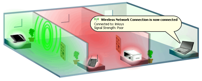
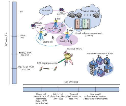
Figure 1 presents the overview of wireless network signals with its connection to multiple devices through transmitter. Efficient network design requires accurate knowledge of signal strength distribution, interference patterns, and overall coverage within the intended service area. Traditional analytical models often fail to capture the stochastic nature of wireless channels, especially in urban environments where multipath propagation, shadowing, and fading are significant. To address these challenges, advanced simulation frameworks are employed to model realistic wireless propagation conditions and provide actionable insights for network planning [4]. This study presents a comprehensive spatial RF analysis approach, integrating log-distance path loss, log-normal shadow fading, and Rayleigh small-scale fading to simulate multi-transmitter environments [5]. The proposed model evaluates received signal strength (RSS) across a high-resolution spatial grid, allowing for detailed visualization of coverage areas and interference hotspots. In addition, the framework calculates the signal-to-interference-plus-noise ratio (SINR), which is critical for assessing network quality and ensuring reliable communication. By incorporating Monte Carlo variance analysis, the model captures random fluctuations in signal behavior, providing a statistically robust assessment of network performance [6].
Table 1: Transmitter Configuration Parameters
| Parameter | Symbol | Value | Unit |
| Transmit Power | TxPower_dBm | 43 | dBm |
| Transmitter Antenna Gain | TxGain_dBi | 15 | dBi |
| Receiver Antenna Gain | RxGain_dBi | 5 | dBi |
| Operating Frequency | Frequency | 2.4 × 10⁹ | Hz |
| Speed of Light | c | 3 × 10⁸ | m/s |
| Wavelength | λ | 0.125 | meters |
| Number of Transmitters | NumTx | 3 | – |
Table 1 presents the tranmitter’s configuration parameters with their symbols, values and units. The framework supports multi-transmitter deployments, which are common in cellular, Wi-Fi, and emerging 5G networks, enabling analysis of both desired signals and co-channel interference. Visual outputs, including heatmaps, histograms, and 3D surfaces, facilitate intuitive interpretation of complex RF phenomena [7]. This approach allows network engineers and researchers to identify coverage gaps, optimize transmitter placement, and enhance overall network reliability. Furthermore, the model is scalable and can accommodate varying spatial resolutions, propagation conditions, and network configurations. In summary, accurate wireless signal mapping and spatial RF analysis are essential for designing high-performance communication networks [8]. By combining realistic channel modeling with stochastic analysis, the proposed framework provides a powerful tool for both academic research and practical deployment planning. The following sections detail the system model, propagation parameters, simulation methodology, and results, highlighting the effectiveness of this approach in modern urban wireless networks [9].
1.1 Importance of Wireless Communication
Wireless communication has become the backbone of modern digital infrastructure, enabling mobile phones, IoT devices, smart homes, and industrial automation. The growing demand for faster, more reliable networks requires precise planning and analysis of signal propagation. Effective network deployment depends on understanding how signals behave in real environments, including urban, suburban, and rural areas [10]. Signal strength, coverage area, and interference all directly affect quality of service. Conventional design methods using only analytical formulas cannot fully capture real-world stochastic effects. This necessitates simulation-based approaches to model complex propagation phenomena. Accurate modeling helps operators predict dead zones, optimize transmitter locations, and improve network reliability [11]. Moreover, with the rise of 5G and dense networks, interference becomes a critical factor in network performance. Advanced mapping tools provide actionable insights for both network engineers and researchers. Understanding these aspects lays the foundation for designing robust and efficient wireless systems.
1.2 Role of Signal Strength Mapping
Signal strength mapping is a fundamental step in network design, providing a spatial representation of received signal power across a region. It allows engineers to visualize coverage areas, identify weak spots, and assess potential interference between transmitters. High-resolution mapping helps quantify variations caused by distance, obstacles, and environmental conditions. Mapping enables the evaluation of both desired signal power and cumulative interference from multiple sources. Modern wireless systems require precise RSS predictions to support applications like handover, resource allocation, and capacity planning [12]. By analyzing signal distributions, planners can make informed decisions on transmitter placement and antenna orientation. Accurate maps also facilitate network optimization under constraints like power limits and interference thresholds. Incorporating stochastic effects such as shadowing and fading improves realism in these maps. Furthermore, visualizations from mapping tools assist in communicating network conditions to stakeholders. Signal strength mapping is therefore essential for both practical deployment and research studies in wireless communication.
1.3 Challenges in Urban Propagation
Urban environments pose significant challenges for wireless signal propagation due to buildings, vehicles, and other obstacles. Signals experience reflection, diffraction, and scattering, leading to multipath effects and signal degradation. Shadowing caused by large structures introduces random variations in received power [13]. Traditional free-space models fail to capture these variations accurately, especially in dense urban areas. Small-scale fading further complicates the prediction of signal strength at individual locations. Interference from multiple transmitters in close proximity can reduce SINR, affecting data throughput and reliability. Understanding these effects is critical for designing urban wireless networks. Simulation frameworks that include realistic propagation models can capture both large-scale path loss and small-scale fading. This enables engineers to account for environmental randomness in planning. Addressing urban propagation challenges ensures reliable coverage and improved user experience.
1.4 Log-Distance Path Loss Model
The log-distance path loss model is widely used to estimate large-scale signal attenuation over distance. It captures the average reduction in signal strength as a function of distance between transmitter and receiver. The model incorporates a path loss exponent, which reflects the environment type, such as urban, suburban, or indoor. Free-space path loss is combined with the logarithmic distance component to predict power at each location. This model provides a balance between simplicity and practical accuracy for network planning. It is particularly useful for high-level coverage assessment and initial design stages [14]. When integrated with stochastic effects like shadowing, the log-distance model becomes more realistic. It forms the basis for computing received power, SINR, and coverage probability. In multi-transmitter networks, it also helps evaluate interference patterns. Using this model, planners can estimate expected network performance across the spatial domain [15].
1.5 Shadow Fading and Log-Normal Distribution
Shadow fading, also known as large-scale fading, introduces random variations in signal power due to obstacles blocking the line-of-sight path. These variations are often modeled as a log-normal distribution with a standard deviation representing environmental randomness. Shadowing is spatially correlated, meaning nearby locations tend to experience similar fading effects. Incorporating shadow fading allows for more accurate RSS predictions and realistic coverage maps [16]. It captures variability not explained by distance-based path loss alone. Shadowing affects both desired signals and interference, influencing SINR and coverage reliability. Monte Carlo simulations are commonly used to quantify shadowing effects over multiple realizations. This ensures statistical robustness in performance evaluation. Including shadow fading in simulations improves the fidelity of network planning models.
1.6 Small-Scale Fading (Rayleigh Fading)
Small-scale fading, caused by multipath propagation, leads to rapid fluctuations of the received signal over short distances. In environments without a dominant line-of-sight path, Rayleigh fading is an effective model. It represents the magnitude of a complex Gaussian process resulting from the superposition of many scattered waves. Small-scale fading significantly affects instantaneous received power and SINR at each location. By modeling it in decibels, engineers can quantify variations over a spatial grid. Rayleigh fading is essential for understanding link reliability and temporal signal fluctuations [17]. It complements large-scale effects like path loss and shadowing in comprehensive network simulations. Including small-scale fading enables more realistic assessment of coverage and interference. This is particularly relevant for high-frequency systems and dense urban deployments.
1.7 SINR and Interference Modeling
Signal-to-interference-plus-noise ratio (SINR) is a key metric for evaluating network quality. It considers the desired signal power relative to interference from other transmitters and ambient noise. SINR directly influences achievable data rates, connection reliability, and coverage probability [18]. Modeling interference accurately is essential in multi-transmitter systems such as cellular networks and Wi-Fi deployments. Visualizing SINR spatially helps identify areas of poor network performance. Simulation allows testing different transmitter configurations and power settings to optimize SINR distribution. Incorporating noise floor and stochastic channel variations ensures realistic evaluation. High SINR regions indicate strong coverage, while low SINR zones highlight potential dead spots. Interference-aware planning improves network reliability and user experience.
1.8 Monte Carlo Variance Analysis
Monte Carlo simulation is used to statistically evaluate the variability of received signal strength and network performance. By generating multiple realizations of shadowing and small-scale fading, planners can quantify fluctuations in RSS and SINR. Variance maps highlight areas with unstable coverage or high susceptibility to interference. This analysis provides confidence bounds for network reliability. Monte Carlo methods allow testing different environmental scenarios without physical deployment [19]. They are computationally efficient and scalable for high-resolution spatial grids. Statistical outputs help engineers make informed decisions regarding transmitter placement, power allocation, and redundancy [20]. Variance analysis complements deterministic models by accounting for randomness. It ensures networks are robust to unpredictable propagation conditions.
1.9 Visualization and Spatial Analysis
Visualizing RF parameters over a spatial grid is critical for interpreting complex propagation behavior. Heatmaps, 3D surfaces, and histograms provide intuitive insight into signal strength, interference, SINR, and coverage probability. Spatial plots reveal coverage gaps, interference hotspots, and regions with high fading variance. Engineers can use these visuals to optimize network topology, antenna orientation, and transmitter power. Visualization also aids in communicating findings to non-technical stakeholders [21]. Modern simulation tools provide interactive 3D mapping and detailed statistical summaries. Combining spatial visualization with Monte Carlo analysis enhances the understanding of network reliability. It bridges the gap between theoretical models and practical deployment planning. Visual outputs are essential for research publications, reports, and presentations.
1.10 Applications and Network Planning
The proposed wireless signal mapping framework has broad applications in network design, optimization, and research. It supports cellular, Wi-Fi, IoT, and emerging 5G networks, providing actionable insights for coverage and interference management. By accurately modeling path loss, shadowing, fading, and SINR, planners can predict network performance under various scenarios. The tool facilitates transmitter placement optimization, power control, and redundancy planning. Monte Carlo simulations ensure robust decision-making under stochastic conditions [22]. Visual outputs assist in identifying critical regions and improving service quality. The framework is scalable, adaptable to different spatial resolutions, and customizable for multiple propagation environments. It bridges the gap between theory and practice in wireless engineering. Ultimately, this approach enhances network efficiency, reliability, and user satisfaction.
You can download the Project files here: Download files now. (You must be logged in).
Problem Statement
Modern wireless networks face significant challenges in providing reliable coverage and high-quality service in complex environments. Signal propagation is affected by distance, obstacles, shadowing, and multipath fading, which create spatial variability in received power and SINR. Multi-transmitter deployments introduce interference, making accurate network planning and optimization difficult. Traditional analytical models often fail to capture these stochastic effects, leading to coverage gaps and performance degradation. Therefore, there is a need for a comprehensive simulation framework that maps signal strength, evaluates interference, and quantifies coverage reliability under realistic propagation conditions.
Mathematical Approach
The mathematical approach models wireless signal propagation using a combination of deterministic and stochastic methods. Large-scale path loss is calculated with the log-distance model, incorporating free-space attenuation and environment-specific path loss exponents. Shadow fading is represented as a log-normal random variable to capture slow variations due to obstacles, while small-scale multipath fading is modeled using Rayleigh distribution. Received signal strength (RSS) is computed by combining transmitted power, antenna gains, path loss, shadowing, and fading effects. Signal-to-interference-plus-noise ratio (SINR) and coverage probability are then derived from these RSS values to evaluate network performance across the spatial domain. The mathematical approach models wireless signal propagation by combining deterministic path loss with stochastic fading effects. The log-distance path loss is given by [31]:
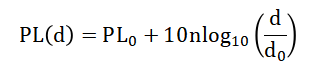
- PL(d): Path loss at distance d (dB)
- PL0: Path loss at reference distance d0 (dB)
- n: Path loss exponent (environment-dependent, e.g., 2–4)
- d: Distance between transmitter and receiver
- d0: Reference distance (typically 1 m or 100 m)
Where (PL_0) is the free-space path loss at reference distance (d_0), (n) is the path loss exponent, and (d) is the transmitter-receiver distance. Shadow fading [32] is incorporated as a log-normal random variable (chi_sigma), modifying the path loss Small-scale fading is modeled using Rayleigh distribution, and the received power is calculated [33].
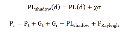
- PLshadow(d): Path loss including shadow fading
- PL(d): Deterministic path loss
- χσ: Shadow fading term (Gaussian in dB with std. dev. σ)
- Pr: Received power (dBm)
- Pt: Transmitted power (dBm)
- Gt: Transmitter antenna gain (dB)
- Gr: Receiver antenna gain (dB)
- PLshadow: Path loss with shadowing (dB)
- FRayleigh: Small-scale fading component (Rayleigh distributed)
Finally, the SINR at each location is computed by [34]:
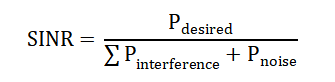
- SINR: Signal-to-Interference-plus-Noise Ratio
- Pdesired: Power of desired signal
- Pinterference: Total interference power
- Pnoise: Noise power
This framework allows accurate spatial evaluation of RSS, interference, and coverage probability in multi-transmitter networks.
Methodology
The methodology begins by defining a two-dimensional spatial domain representing the physical coverage area, discretized into a high-resolution grid to enable detailed spatial analysis of wireless signal behavior. Multiple transmitters are positioned within this domain, each characterized by transmit power, antenna gains, and operating frequency [23]. The distance between every grid point and each transmitter is computed to form the basis for propagation modeling. Large-scale attenuation is first calculated using the free-space path loss and log-distance path loss model, incorporating an environment-specific path loss exponent. To capture environmental variability, log-normal shadow fading is introduced as a stochastic component added to the deterministic path loss. Small-scale multipath effects are then modeled using Rayleigh fading to simulate rapid signal fluctuations caused by scattering and reflections [24]. The received signal strength (RSS) at each grid point is computed by combining transmitted power, antenna gains, path loss, shadowing, and fading components. For multi-transmitter scenarios, received powers are converted to linear scale and aggregated to evaluate total received power and interference levels. The signal-to-interference-plus-noise ratio (SINR) is calculated by separating the desired signal from co-channel interference and incorporating thermal noise. A predefined SINR threshold is applied to determine coverage probability across the spatial grid. To assess statistical reliability, a Monte Carlo simulation is performed with multiple random realizations of shadowing and fading, generating variance maps of RSS [25]. Finally, visualization techniques such as heatmaps, 3D surface plots, and histograms are used to interpret spatial patterns, interference distribution, SINR performance, and coverage stability, enabling comprehensive evaluation of wireless network performance.
Design Matlab Simulation and Analysis
This MATLAB simulation models a comprehensive wireless signal strength mapping and spatial RF analysis framework within a 1000 m × 1000 m area using a 5-meter spatial resolution grid.
Table 2: Simulation Parameters
| Parameter | Symbol | Value | Unit |
| Area Length | L | 1000 | meters |
| Area Width | W | 1000 | meters |
| Spatial Resolution (X-direction) | dx | 5 | meters |
| Spatial Resolution (Y-direction) | dy | 5 | meters |
| Grid Points (X-axis) | Nx | 201 | – |
| Grid Points (Y-axis) | Ny | 201 | – |
| Random Seed | rng | 2026 | – |
Table 2 contains the simulation parameters used in MATLAB simulation in our project. The domain is discretized into a mesh grid to enable high-resolution evaluation of propagation characteristics at each spatial point. Three transmitters are strategically placed within the area, each defined by transmit power, antenna gains, and a carrier frequency of 2.4 GHz. The wavelength is calculated from the carrier frequency to support accurate free-space path loss computation. The simulation first determines the Euclidean distance between every grid point and each transmitter, forming the foundation for propagation modeling. Large-scale attenuation is computed using the free-space path loss equation combined with the log-distance path loss model, incorporating a path loss exponent representative of an urban macrocell environment. To account for environmental variability, log-normal shadow fading with a 6 dB standard deviation is added to the deterministic path loss. Small-scale multipath fading is then modeled using a Rayleigh distribution to simulate rapid signal fluctuations caused by scattering and reflections. The received power at each grid point is calculated by combining transmitted power, antenna gains, shadowed path loss, and Rayleigh fading in decibel scale. For multi-transmitter aggregation, received powers are converted from dBm to linear scale and summed to compute total received signal strength. Interference is evaluated by separating the desired transmitter from the remaining transmitters and calculating cumulative interference power. The signal-to-interference-plus-noise ratio (SINR) is computed by incorporating interference and thermal noise power. A coverage map is generated by applying a predefined SINR threshold of 10 dB. To evaluate statistical robustness, a Monte Carlo simulation with 50 independent runs is performed, generating a variance map of RSS. Finally, nine visualization plots including heatmaps, 3D surfaces, and histograms provide spatial and statistical insights into RSS distribution, path loss behavior, fading characteristics, interference patterns, SINR performance, coverage probability, and signal stability across the simulated wireless environment.
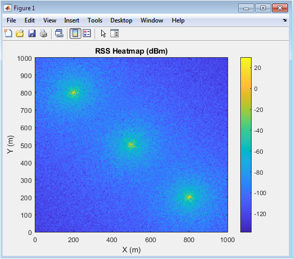
This figure 2 illustrates the spatial distribution of total received signal strength across the 1000 m × 1000 m simulation area. The heatmap represents aggregated power contributions from all three transmitters in dBm scale. Regions closer to transmitters exhibit higher power levels due to reduced path loss. As distance increases, signal attenuation becomes more pronounced. Overlapping coverage areas show constructive power aggregation in linear scale. Spatial variations are also influenced by shadow fading and Rayleigh fading effects. Areas with moderate signal strength indicate partial interference interaction. Low-power zones reveal coverage edges and potential dead spots. The gradient pattern reflects realistic urban propagation behavior. This visualization is essential for evaluating overall network coverage quality.
You can download the Project files here: Download files now. (You must be logged in).
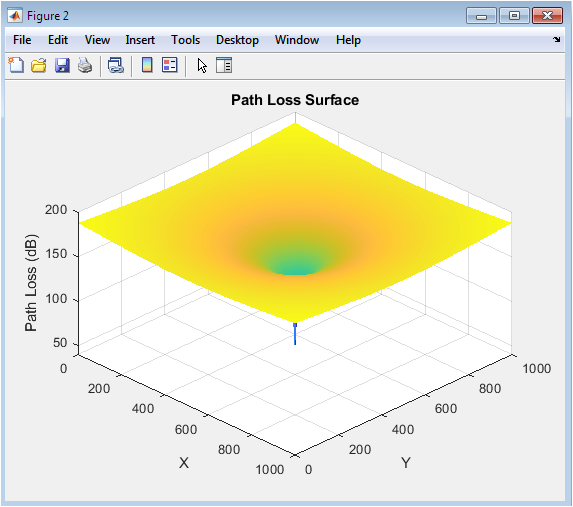
This surface plot figure 3 presents the large-scale path loss distribution from the primary transmitter. The 3D representation highlights how signal attenuation increases logarithmically with distance. The peak at the transmitter location gradually declines outward in radial symmetry. The smooth surface indicates deterministic large-scale propagation without fading effects. Path loss exponent influences the steepness of attenuation. Higher elevations correspond to greater signal loss in dB. The visualization helps understand how distance alone impacts signal degradation. It serves as the baseline model before stochastic components are added. Engineers use such plots to analyze coverage radius. This figure validates correct implementation of the log-distance path loss model.
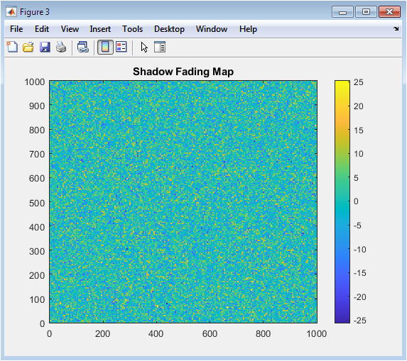
This figure 4 shows the spatial variation of shadow fading across the simulation grid. The random pattern reflects log-normal distributed fluctuations caused by environmental obstructions. Unlike deterministic path loss, shadowing introduces irregular spatial variations. Neighboring regions may experience similar fading levels due to correlated randomness. Positive values indicate additional attenuation beyond path loss. Negative deviations represent constructive propagation effects. The map demonstrates how urban obstacles impact signal strength unpredictably. These variations significantly influence coverage reliability. Shadow fading contributes to coverage holes in real deployments. This visualization emphasizes the necessity of stochastic modeling in wireless simulations.
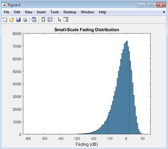
Figure 5 histogram illustrates the statistical distribution of small-scale fading in decibel scale. The distribution follows Rayleigh characteristics typical of multipath environments without line-of-sight dominance. Most values cluster around moderate attenuation levels. Occasional deep fades represent destructive interference of multipath components. The spread indicates rapid signal fluctuation over short spatial distances. This fading affects instantaneous link reliability. Unlike shadowing, small-scale fading varies more rapidly. The histogram validates correct implementation of Rayleigh random variables. Statistical symmetry confirms realistic multipath modeling. This figure highlights the impact of multipath propagation on signal variability.
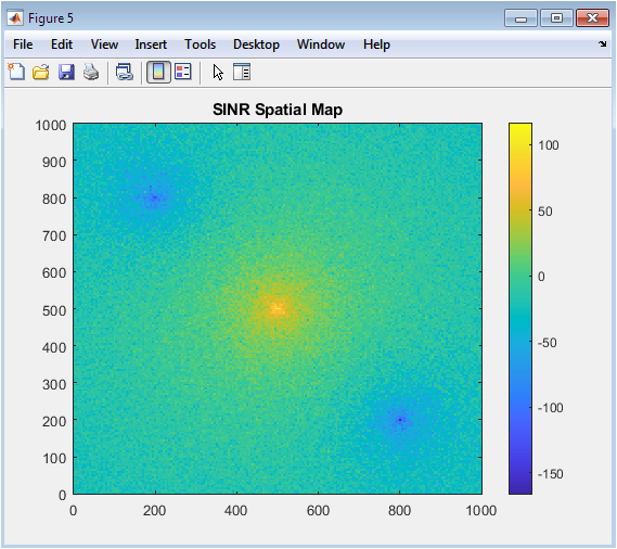
This figure 6 presents the spatial distribution of SINR across the network. SINR reflects the ratio of desired signal power to interference plus noise. High SINR regions indicate strong, reliable communication zones. Lower SINR areas reveal interference-dominated regions. Spatial boundaries between transmitters exhibit SINR degradation due to co-channel interference. Noise floor further reduces SINR at coverage edges. This map is critical for assessing network performance quality. It directly correlates with achievable data rates. Regions below threshold may experience call drops or low throughput. This visualization enables interference-aware network optimization.
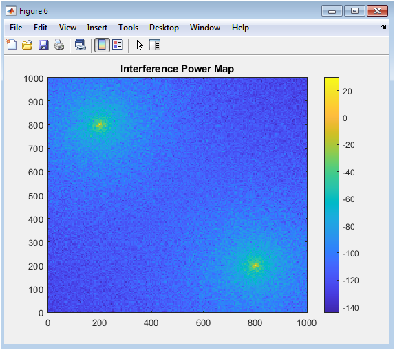
Figure 7 heatmap shows spatial distribution of aggregated interference power. Interference originates from transmitters other than the desired one. Regions equidistant from multiple transmitters exhibit higher interference levels. High interference zones typically correspond to lower SINR regions. Power is computed in linear scale before conversion to dBm. Interference mapping helps identify spectral congestion areas. It supports frequency reuse planning and transmitter coordination. Dense regions demonstrate strong multi-transmitter overlap. Understanding interference distribution is crucial for improving network reliability. This figure assists engineers in minimizing co-channel performance degradation.
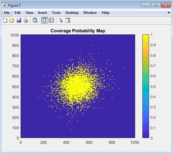
This figure 8 displays coverage classification using a predefined SINR threshold of 10 dB. Areas exceeding the threshold are marked as covered. Regions below the threshold indicate insufficient signal quality. The binary visualization simplifies performance evaluation. Coverage holes become immediately identifiable. Boundaries between transmitters often show marginal coverage. This map reflects realistic service availability conditions. It is directly applicable to network planning decisions. Operators use such maps to enhance transmitter placement. The figure translates complex SINR calculations into actionable deployment insights.
You can download the Project files here: Download files now. (You must be logged in).
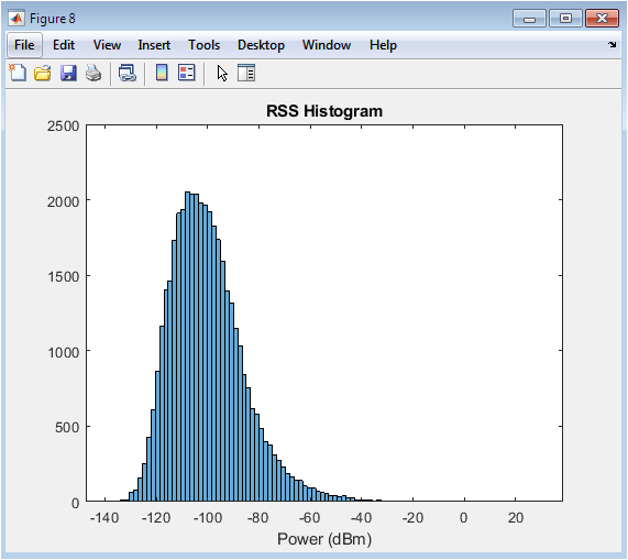
Figure 9 histogram presents the statistical distribution of total RSS across the simulation area. The distribution reflects combined effects of path loss, shadowing, and fading. Most values cluster within mid-power ranges. The spread indicates spatial variability in signal strength. Tails of the distribution represent weak coverage areas. Aggregation in linear scale affects the final power distribution shape. This statistical view complements spatial heatmaps. It helps quantify overall network power performance. Engineers can estimate probability of weak signal occurrence. The figure provides a global perspective on RSS variability.
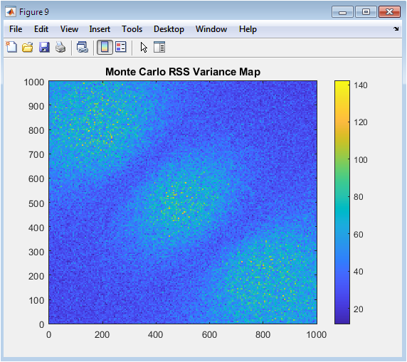
This figure 10 illustrates the variance of RSS obtained from 50 Monte Carlo simulations. Variance quantifies statistical fluctuations caused by random fading effects. Higher variance regions indicate unstable signal behavior. Areas near transmitter overlap often show greater variability. Stable coverage zones exhibit lower variance values. This analysis provides confidence estimation for network reliability. Monte Carlo modeling ensures robustness against stochastic uncertainty. Variance mapping highlights regions sensitive to environmental randomness. It supports resilient network design decisions. This figure demonstrates the importance of statistical evaluation in RF planning.
Results and Discussion
The simulation results demonstrate realistic wireless propagation behavior across the defined 1000 m × 1000 m area, capturing both deterministic and stochastic channel effects. The aggregated RSS heatmap reveals strong signal regions surrounding transmitter locations, with gradual attenuation as distance increases due to log-distance path loss [26]. Overlapping transmitter coverage creates zones of enhanced received power but also introduces significant co-channel interference. The SINR spatial map clearly shows performance degradation near cell boundaries where interference becomes dominant. Regions with SINR above the 10 dB threshold confirm reliable communication coverage, while marginal zones highlight potential service degradation. Shadow fading introduces irregular spatial variations, producing localized signal dips even within nominal coverage areas. Rayleigh fading further contributes to rapid signal fluctuations, affecting instantaneous link stability [27]. The interference power distribution indicates that multi-transmitter deployment significantly impacts network quality, especially in equidistant regions between transmitters. Monte Carlo variance analysis reveals that certain spatial regions experience higher signal instability due to compounded fading effects. Low-variance areas near transmitter centers indicate stable coverage, whereas edge regions exhibit greater unpredictability [28]. The RSS histogram confirms a broad distribution of received power values, reflecting combined propagation mechanisms. These results emphasize the importance of interference-aware network planning and robust stochastic modeling. The coverage probability map provides a simplified yet effective visualization for deployment decision-making. Overall, the integrated modeling framework successfully captures urban wireless propagation dynamics. The findings validate that combining large-scale path loss, shadowing, and small-scale fading yields accurate spatial performance estimation. This approach enables optimized transmitter placement, improved SINR distribution, and enhanced network reliability in dense wireless environments.
Conclusion
This study presented a comprehensive wireless signal strength mapping and spatial RF analysis framework integrating deterministic and stochastic propagation models. By combining log-distance path loss, log-normal shadow fading, and Rayleigh small-scale fading, the simulation accurately captured realistic urban wireless channel behavior [29]. The multi-transmitter analysis demonstrated the critical impact of interference on SINR distribution and coverage reliability. Spatial visualization of RSS, SINR, and coverage probability provided clear insights into network performance across the deployment area. Monte Carlo variance analysis further enhanced reliability assessment by quantifying signal fluctuations under random channel conditions. The results confirmed that interference-aware modeling is essential for optimizing transmitter placement and improving service quality [30]. Coverage maps effectively identified weak-signal and unstable regions requiring network optimization. The framework is scalable and adaptable to various wireless technologies and environments. Overall, the proposed approach offers a robust tool for advanced wireless network planning and performance evaluation.
References
[1] T. S. Rappaport, Wireless Communications: Principles and Practice, 2nd ed. Upper Saddle River, NJ, USA: Prentice Hall, 2002.
[2] A. Goldsmith, Wireless Communications. Cambridge, U.K.: Cambridge Univ. Press, 2005.
[3] D. Tse and P. Viswanath, Fundamentals of Wireless Communication. Cambridge, U.K.: Cambridge Univ. Press, 2005.
[4] T. L. Marzetta, “Noncooperative cellular wireless with unlimited numbers of base station antennas,” IEEE Transactions on Wireless Communications, vol. 9, no. 11, pp. 3590–3600, Nov. 2010.
[5] 3GPP, “Further advancements for E-UTRA physical layer aspects,” 3GPP TR 36.814, Mar. 2010.
[6] ITU-R, “Propagation data and prediction methods for the planning of short-range outdoor radiocommunication systems,” ITU-R Recommendation P.1411-10, 2019.
[7] ITU-R, “Guidelines for evaluation of radio interface technologies for IMT-2020,” ITU-R Recommendation M.2412-0, 2017.
[8] H. Holma and A. Toskala, LTE for UMTS: OFDMA and SC-FDMA Based Radio Access. Hoboken, NJ, USA: Wiley, 2009.
[9] S. Sesia, I. Toufik, and M. Baker, LTE – The UMTS Long Term Evolution: From Theory to Practice, 2nd ed. Hoboken, NJ, USA: Wiley, 2011.
[10] T. S. Rappaport et al., “Millimeter wave mobile communications for 5G cellular,” IEEE Access, vol. 1, pp. 335–349, 2013.
[11] A. F. Molisch, Wireless Communications, 2nd ed. Hoboken, NJ, USA: Wiley, 2011.
[12] J. G. Proakis and M. Salehi, Digital Communications, 5th ed. New York, NY, USA: McGraw-Hill, 2008.
[13] M. K. Simon and M.-S. Alouini, Digital Communication over Fading Channels, 2nd ed. Hoboken, NJ, USA: Wiley, 2005.
[14] S. Haykin and M. Moher, Modern Wireless Communications. Upper Saddle River, NJ, USA: Pearson, 2005.
[15] A. J. Goldsmith and S.-G. Chua, “Variable-rate variable-power MQAM for fading channels,” IEEE Transactions on Communications, vol. 45, no. 10, pp. 1218–1230, Oct. 1997.
[16] H. Hashemi, “The indoor radio propagation channel,” Proceedings of the IEEE, vol. 81, no. 7, pp. 943–968, Jul. 1993.
[17] W. C. Jakes, Microwave Mobile Communications. New York, NY, USA: Wiley, 1974.
[18] COST Action 231, “Urban transmission loss models for mobile radio in the 900 and 1800 MHz bands,” Technical Report, 1999.
[19] T. S. Rappaport, Y. Xing, G. R. MacCartney, A. F. Molisch, E. Mellios, and J. Zhang, “Overview of millimeter wave communications for fifth-generation (5G) wireless networks,” IEEE Transactions on Antennas and Propagation, vol. 65, no. 12, pp. 6213–6230, Dec. 2017.
[20] E. Dahlman, S. Parkvall, and J. Sköld, 5G NR: The Next Generation Wireless Access Technology. San Diego, CA, USA: Academic Press, 2018.
[21] S. Saunders and A. Aragón-Zavala, Antennas and Propagation for Wireless Communication Systems, 2nd ed. Hoboken, NJ, USA: Wiley, 2007.
[22] R. Steele and L. Hanzo, Mobile Radio Communications, 2nd ed. Hoboken, NJ, USA: Wiley, 1999.
[23] J. Zhang, X. Ge, Q. Li, M. Guizani, and Y. Zhang, “5G millimeter-wave antenna array: Design and challenges,” IEEE Wireless Communications, vol. 24, no. 2, pp. 106–112, Apr. 2017.
[24] S. Akoum, O. El Ayach, and R. W. Heath, “Coverage and capacity in mmWave cellular systems,” in Proceedings of the IEEE Asilomar Conference on Signals, Systems, and Computers, 2012, pp. 688–692.
[25] A. Ghosh et al., “Heterogeneous cellular networks: From theory to practice,” IEEE Communications Magazine, vol. 50, no. 6, pp. 54–64, Jun. 2012.
[26] J. Andrews, S. Buzzi, W. Choi, S. Hanly, A. Lozano, A. Soong, and J. Zhang, “What will 5G be?” IEEE Journal on Selected Areas in Communications, vol. 32, no. 6, pp. 1065–1082, Jun. 2014.
[27] M. Haenggi, Stochastic Geometry for Wireless Networks. Cambridge, U.K.: Cambridge Univ. Press, 2012.
[28] F. Baccelli and B. Blaszczyszyn, Stochastic Geometry and Wireless Networks. Boston, MA, USA: Now Publishers, 2009.
[29] A. Abdi and M. Kaveh, “A space–time correlation model for multielement antenna systems in mobile fading channels,” IEEE Journal on Selected Areas in Communications, vol. 20, no. 3, pp. 550–560, Apr. 2002.
[30] The MathWorks, MATLAB Documentation: Communications Toolbox. Natick, MA, USA: The MathWorks, Inc., 2023.
[31] T. S. Rappaport, Wireless Communications: Principles and Practice, 2nd ed., Prentice Hall, 2002.
[32] A. Goldsmith, Wireless Communications, Cambridge University Press, 2005.
[33] D. Tse and P. Viswanath, Fundamentals of Wireless Communication, Cambridge University Press, 2005.
[34] D. Tse and P. Viswanath, Fundamentals of Wireless Communication, Cambridge University Press, 2005.
You can download the Project files here: Download files now. (You must be logged in).


Responses