

Cellular Network Planning, Interference Management, and Power Optimization Using Matlab Simulation
Author : Waqas Javaid
Abstract
This article provides a comprehensive exploration of an advanced MATLAB-based simulation tool designed for cellular network planning and optimization, breaking down the complex algorithms that underpin modern telecommunications infrastructure. It examines the transition from theoretical hexagonal cell layouts to real-world propagation modeling using the COST-231 Hata model, illustrating how engineers predict signal strength and path loss across diverse environments [1]. The discussion delves into critical quality metrics such as SINR and handover probability, explaining how co-channel interference and user mobility directly impact the Quality of Experience for end-users. Furthermore, it highlights the importance of traffic engineering through the Erlang-B formula and demonstrates how automated power optimization loops, mimicking Self-Organizing Network (SON) capabilities, can dynamically balance network load [2]. Ultimately, the piece serves as a bridge between academic theory and practical engineering, revealing how these foundational principles are applied to ensure seamless connectivity in the 5G era and beyond [3].
Introduction
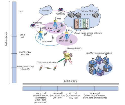
The rapid evolution of wireless communication from 4G to the hyper-connected 5G era has fundamentally transformed the way we design, deploy, and manage cellular networks, introducing unprecedented levels of complexity that render traditional trial-and-error methods obsolete [4].
Figure 1 presents the cellular network planning and optimization in which data consumption skyrockets and user expectations for seamless connectivity intensify, network operators are compelled to move beyond simple coverage maps and embrace sophisticated, data-driven planning methodologies that can predict and mitigate real-world challenges before they impact the end-user [5]. The margin for error has shrunk considerably; a poorly planned cell site today doesn’t just mean a dropped call, but potentially failed autonomous vehicles, interrupted telemedicine procedures, and frustrated users in ultra-dense urban environments [6]. Consequently, modern network planning has evolved into a multidisciplinary science that integrates advanced RF propagation modeling, statistical traffic analysis, and automated optimization algorithms to ensure robust performance. At the heart of this discipline lies the need to balance conflicting objectives: maximizing coverage while minimizing interference, accommodating explosive traffic growth while maintaining quality of service, and ensuring user mobility without sacrificing connection stability [7]. Engineers are tasked with solving intricate puzzles involving frequency reuse, power control, and handover management, often across heterogeneous landscapes that include sprawling suburban areas and dense metropolitan canyons. To navigate these complexities, the industry relies heavily on computational simulation tools that can model thousands of user interactions, base station configurations, and environmental variables in a controlled, repeatable manner [8]. These tools serve as virtual proving grounds where theoretical concepts such as hexagonal cell planning, the COST-231 Hata propagation model, and the Erlang-B traffic formula are stress-tested against realistic interference scenarios. By simulating the intricate dance between mobile users and base stations, engineers can visualize SINR distributions, identify coverage holes, and optimize handover parameters long before a single tower is erected. This proactive approach not only slashes capital expenditure by preventing costly design flaws but also ensures that networks are resilient enough to handle the unpredictable nature of human mobility and traffic demand [9]. This article aims to demystify these processes by conducting a deep dive into an advanced cellular network planning and optimization tool built in MATLAB, exploring how each module from user association to power control contributes to the creation of a high-performance wireless ecosystem [10]. By understanding these foundational principles, readers will gain valuable insight into the invisible infrastructure that powers our connected world and the engineering ingenuity required to keep us all online.
1.1 The New Reality of Wireless Connectivity
The rapid evolution of wireless communication from 4G to the hyper-connected 5G era has fundamentally transformed the way we design, deploy, and manage cellular networks. This shift introduces unprecedented levels of complexity that render traditional trial-and-error methods completely obsolete for modern infrastructure projects. As data consumption skyrockets and user expectations for seamless connectivity intensify, network operators are compelled to embrace sophisticated, data-driven planning methodologies [11]. These advanced approaches are necessary to predict and mitigate real-world challenges before they negatively impact the end-user experience. The margin for error has shrunk considerably, making precision engineering a non-negotiable requirement in the telecommunications industry.
1.2 The High Stakes of Network Failure
A poorly planned cell site today doesn’t just mean a single dropped call for a subscriber, but carries far more severe consequences in our interconnected world. Such failures could potentially lead to failed autonomous vehicle communications, interrupted telemedicine procedures requiring immediate connectivity, and frustrated users in ultra-dense urban environments where network congestion is rampant [12]. These failures erode consumer trust and can have serious safety implications in critical applications. The financial repercussions are equally significant, as operators face costly remediation efforts and potential loss of subscribers to competitors. Therefore, the quality of initial network planning directly impacts both public safety and corporate profitability.
1.3 The Multidisciplinary Nature of Modern Planning
Consequently, modern network planning has evolved into a sophisticated multidisciplinary science that integrates advanced RF propagation modeling with statistical traffic analysis. It also relies heavily on automated optimization algorithms that continuously fine-tune parameters to ensure robust performance across diverse scenarios [13]. This integration allows engineers to simulate complex interactions between physical infrastructure and user behavior with remarkable accuracy. The discipline draws knowledge from electrical engineering, computer science, and applied mathematics to solve real-world communication challenges [14]. By combining these fields, planners can create networks that are both technically excellent and economically viable to operate.
1.4 The Fundamental Balancing Act
At the heart of this discipline lies the intricate challenge of balancing multiple conflicting objectives that define network performance. Engineers must maximize coverage area while simultaneously minimizing co-channel interference that degrades signal quality for everyone. They are tasked with accommodating explosive traffic growth driven by video streaming and IoT devices while maintaining strict quality of service standards [15]. The network must also ensure seamless user mobility across cell boundaries without sacrificing connection stability during handovers. This delicate balancing act requires constant monitoring and adjustment as usage patterns evolve throughout the day.
1.5 Solving Complex Engineering Puzzles
Engineers are tasked daily with solving intricate puzzles involving frequency reuse patterns that maximize spectral efficiency across their networks. They must implement sophisticated power control mechanisms that prevent one tower from overwhelming neighboring cells with excessive signal strength. Handover management algorithms must be carefully tuned to ensure users moving at high speeds maintain uninterrupted connectivity [16]. These challenges are compounded when networks must serve heterogeneous landscapes that include sprawling suburban neighborhoods and dense metropolitan canyons. Each environment presents unique propagation characteristics that demand customized engineering solutions rather than one-size-fits-all approaches [17].
1.6 The Role of Computational Simulation
To navigate these complexities effectively without disrupting live services, the industry relies heavily on computational simulation tools that model thousands of user interactions. These platforms can simulate countless base station configurations and environmental variables in a controlled, repeatable manner that would be impossible in the field. Engineers can test extreme scenarios, such as stadium events or natural disasters, to ensure network resilience under peak stress conditions [18]. Simulations allow for rapid iteration and optimization without the enormous cost of physical tower modifications. This virtual approach accelerates innovation cycles while minimizing risk to existing infrastructure investments.
1.7 Virtual Testing Grounds for Theory
These sophisticated tools serve as virtual proving grounds where theoretical concepts such as hexagonal cell planning are validated against realistic conditions. Foundational models like the COST-231 Hata propagation formula can be stress-tested alongside the Erlang-B traffic equation in complex interference scenarios. Engineers can observe how frequency reuse factors perform when subjected to real-world terrain variations and building densities [19]. The controlled environment of simulation allows for isolation of specific variables to understand their individual impact on system performance. This bridges the gap between textbook knowledge and practical application in live network environments.
1.8 Visualizing Invisible Network Dynamics
By simulating the intricate dance between mobile users and base stations, engineers can visualize SINR distributions across entire cities to identify problematic weak spots. They can pinpoint coverage holes that would otherwise remain invisible until subscribers complain about poor service quality. Handover parameters can be optimized by observing exactly how users transition between cells along major transportation routes [20]. This visualization capability transforms abstract mathematical concepts into actionable insights for network optimization teams. Engineers can literally see the invisible radio waves and make data-driven decisions about infrastructure placement.
1.9 Economic Benefits of Proactive Planning
This proactive approach to network design not only slashes capital expenditure by preventing costly design flaws before construction begins. It ensures that networks are resilient enough to handle the unpredictable nature of human mobility and fluctuating traffic demand patterns. Operators can right-size their infrastructure investments based on accurate predictive models rather than conservative overbuilding [21]. The ability to identify and fix issues in simulation saves millions in avoided truck rolls and emergency tower modifications. This financial efficiency ultimately translates to more affordable service prices for end consumers.
1.10 Article Objectives and Scope
This article aims to demystify these complex processes by conducting a deep dive into an advanced cellular network planning and optimization tool built in the MATLAB environment. We will explore how each functional module, from initial user association algorithms to closed-loop power control systems, contributes to creating a high-performance wireless ecosystem [22]. By understanding these foundational principles, readers will gain valuable insight into the invisible infrastructure that powers our connected world. The engineering ingenuity required to keep billions of devices online simultaneously becomes apparent through this detailed examination. Ultimately, this exploration reveals the remarkable complexity hidden beneath the simple act of streaming a video or making a phone call.
Problem Statement
Designing and deploying modern cellular networks has become an increasingly complex challenge, as engineers must balance the conflicting objectives of maximizing coverage, minimizing co-channel interference, and ensuring seamless user mobility across cell boundaries. Traditional planning methods often fail to accurately predict real-world performance, leading to costly over-provisioning of infrastructure or, conversely, the emergence of problematic coverage holes and capacity bottlenecks that degrade the Quality of Experience for subscribers. Furthermore, the dynamic nature of user traffic and the stochastic behavior of interference make it nearly impossible to optimize key parameters like base station transmit power and handover thresholds using static, rule-of-thumb calculations. Without a robust framework for modeling propagation characteristics, analyzing traffic load using tools like the Erlang-B formula, and simulating interference scenarios, network operators risk deploying systems that are inefficient, unreliable, and ill-equipped to handle the demands of high-density urban environments. Therefore, there is a critical need for an integrated simulation tool that can model these complex interactions, visualize key performance indicators, and automate the optimization of network parameters to ensure robust and reliable connectivity.
Mathematical Approach
The mathematical foundation of this cellular network planning tool begins with the (COST-231 Hata path loss model) [31], which predicts signal degradation as where received power [31] is derived enabling the calculation of the Signal-to-Interference-plus-Noise Ratio (SINR) [32] for each user as to quantify link quality.
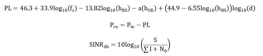
- PL: Path loss (dB)
- fc: Carrier frequency (MHz)
- hBS: Base station antenna height (m)
- hUE: User equipment (mobile) antenna height (m)
- a(hUE): Mobile antenna height correction factor
- d: Distance between transmitter and receiver (km)
- Prx: Received power (dBm)
- Ptx: Transmitted power (dBm)
- PL: Path loss (dB)
- SINRdB: SINR in decibels
- S: Signal power
- I: Interference power
- N0: Noise power
Network capacity and congestion are assessed using the Erlang-B formula [33], which models the probability of call blocking given offered traffic (A) and available channels (m), while handover probability is modeled as a function of SINR degradation [34] using for users below the QoS threshold.
- B(A,m): Blocking probability (probability a call is rejected)
- A: Offered traffic load (in Erlangs)
- mmm: Number of available servers/channels
- k: Summation index (number of occupied channels)
- m!: Factorial of m
- PHO: Handover / outage probability
- β: System-dependent parameter (e.g., fading or network density factor)
- γth: SINR threshold
- γ: Instantaneous SINR
- e(.): Exponential function
Finally, system optimization is achieved through an iterative gradient descent algorithm, which minimizes a cost function by dynamically adjusting base station transmit powers to balance coverage and interference [35].
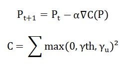
- Pt+1: Updated transmit power vector for next iteration
- Pt: Current transmit power vector at iteration t
- α: Learning rate (step size controlling convergence speed)
- ∇C(P): Gradient of cost function Cwith respect to power P
- C: Cost function value for optimization
- γth: SINR threshold (minimum acceptable Signal-to-Interference-plus-Noise Ratio)
- γu: Instantaneous SINR at user u
- max(0,): Hinge function (zero when SINR meets threshold, positive otherwise)
The mathematical modeling begins with the COST-231 Hata path loss equation, which calculates how much the signal weakens as it travels from the base station to the user, taking into account the carrier frequency, the height of the base station antenna, the height of the user device, and the distance between them. This path loss value is then subtracted from the known transmit power of the base station to determine the actual received signal power at the user’s location, which forms the basis for all subsequent quality calculations. Using these received power values, the simulation computes the Signal-to-Interference-plus-Noise Ratio for each user by comparing the power received from their serving base station against the sum of interference from all other base stations plus the ambient noise floor. To predict network capacity and the likelihood of congestion, the tool employs the Erlang-B formula, which models a telephone system where calls arrive randomly and are either served immediately if a channel is free or blocked entirely if all channels are occupied. This formula calculates the probability of blocking based on the total offered traffic load, measured in Erlangs, and the finite number of channels available at each base station. The simulation also models user mobility challenges by calculating handover probability, which increases exponentially as a user’s signal quality drops below the minimum acceptable threshold, reflecting the likelihood that the device will need to switch to a neighboring cell. When the network requires optimization, the tool implements a gradient descent algorithm that iteratively adjusts the transmit power of every base station to improve overall performance. This optimization process works by defining a cost function that sums up the squared penalties for all users whose signal quality falls below the required threshold, creating a mathematical representation of network dissatisfaction. At each iteration, the algorithm estimates the gradient, or the direction of steepest ascent, of this cost function and takes a small step in the opposite direction to reduce the total cost. Through repeated iterations, this mathematical approach systematically fine-tunes base station powers to strike an optimal balance between providing strong coverage to users and minimizing harmful interference between neighboring cells.
Methodology
The simulation methodology begins by establishing the physical layout of the network, where base stations are placed in a hexagonal grid pattern spanning multiple tiers to create a realistic cellular topology with consistent frequency reuse distances. Following the infrastructure deployment, a large population of user equipment is randomly distributed across the coverage area to simulate a dense urban environment with varied spatial distribution [23].
Table 1: Path Loss Model Parameters (COST-231 HATA)
| Parameter | Symbol | Value | Unit | Formula/Description |
| Base Station Height | h_BS | 30 | m | Antenna height above ground |
| User Equipment Height | h_UE | 1.5 | m | Mobile device height |
| Mobile Antenna Correction Factor | a(h_UE) | (1.1log₁₀f_c – 0.7)h_UE – (1.56log₁₀f_c – 0.8) | dB | Urban environment correction |
| Path Loss at Distance d | PL(d) | 46.3 + 33.9log₁₀f_c – 13.82log₁₀h_BS – a(h_UE) + (44.9 – 6.55log₁₀h_BS)log₁₀d | dB | COST-231 Hata model |
| Distance Range | d | 0.001 – 2.5 | km | BS-UE separation |
Table 1 provide us a path loss model parameters with its values and units used in our paper. The core propagation analysis is then performed using the COST-231 Hata model, which calculates the path loss between every user and every base station by accounting for carrier frequency, antenna heights, and the Euclidean distance between each pair. From these path loss values, the received signal power at each user from every base station is derived, creating a complete power matrix that represents the RF landscape of the simulated network. Each user is then associated with the base station that provides the strongest received signal power, establishing the initial serving cell assignments that determine coverage boundaries and cell edges. The SINR for every user is subsequently calculated by treating the power from the serving cell as the desired signal, summing the power from all other base stations as co-channel interference, and adding the system noise floor to account for thermal and receiver noise contributions [24]. To model realistic network usage patterns, traffic analysis is conducted using the Erlang-B formula, which computes blocking probabilities based on the offered traffic load and the finite channel capacity available at each base station. Handover probability is then assessed for each user based on their current SINR relative to a predefined quality threshold, with users experiencing poor signal quality showing exponentially higher likelihood of needing to transition to a neighboring cell. The optimization phase employs an iterative gradient descent algorithm that adjusts the transmit power of every base station to minimize a cost function representing the total quality-of-service violations across all users [25]. Finally, the methodology concludes with comprehensive visualization of all computed metrics, including received power maps, SINR distributions, traffic loads, handover probabilities, and optimization convergence curves, providing a holistic view of network performance.
You can download the Project files here: Download files now. (You must be logged in).
Design Matlab Simulation and Analysis
The simulation begins by defining all system parameters, including carrier frequency, transmit power, bandwidth, and noise figure, before establishing a hexagonal grid of base stations arranged in multiple tiers to create a realistic cellular topology with consistent spacing.
Table 2: System Parameters and Configuration
| Parameter | Symbol | Value | Unit | Description |
| Carrier Frequency | fc | 1800 | MHz | Operating frequency band |
| Transmit Power | Pt_dBm | 43 | dBm | Initial BS transmission power |
| System Bandwidth | BW | 10 | MHz | Available spectrum |
| Noise Figure | NF | 5 | dB | Receiver noise figure |
| Noise Power | N0 | -174 + 10log₁₀(BW) + NF | dBm | Thermal noise floor |
| Cell Radius | R | 500 | m | Hexagonal cell coverage radius |
| Number of Tiers | N_tiers | 2 | – | Hexagonal deployment layers |
| Frequency Reuse Factor | K | 3 | – | Resource allocation pattern |
| Number of Users | U | 1000 | – | Active subscribers |
| QoS SINR Threshold | SINR_min | 5 | dB | Minimum acceptable SINR |
In the table 2 we have added system parameters and its configuration used in our simulation. A population of one thousand users is then randomly distributed across the coverage area, and the COST-231 Hata path loss model is applied to calculate the signal attenuation between every user and every base station, accounting for antenna heights and distances to generate a complete path loss matrix. From these path loss values, the received signal power at each user from every base station is computed by subtracting the path loss from the transmit power, and each user is associated with the base station providing the strongest signal. The simulation then calculates the Signal-to-Interference-plus-Noise Ratio for every user by treating the power from the serving base station as the desired signal, summing the power from all other base stations as co-channel interference, and adding the system noise floor to the denominator. Traffic modeling is performed using the Erlang-B formula to compute blocking probability based on call arrival rates and holding times, while the actual traffic load per cell is determined by counting how many users are associated with each base station. Handover probability is assessed for users with poor signal quality, modeled as an exponential function of how far their SINR falls below the minimum quality threshold [26]. The core optimization routine then executes forty iterations of a gradient descent algorithm that adjusts the transmit power of every base station, recalculating SINR at each step to evaluate a cost function representing total quality violations. An approximate random gradient is used to update the power values, gradually reducing the cost and improving overall network performance through successive iterations. Finally, the simulation generates eight visualization figures that graphically represent the hexagonal layout, received power map, path loss distribution, SINR values, user associations, traffic loads, handover probabilities, and the convergence of the optimization algorithm. The entire process demonstrates how computational tools can model complex RF interactions, predict network performance metrics, and automatically optimize system parameters to enhance cellular network quality.
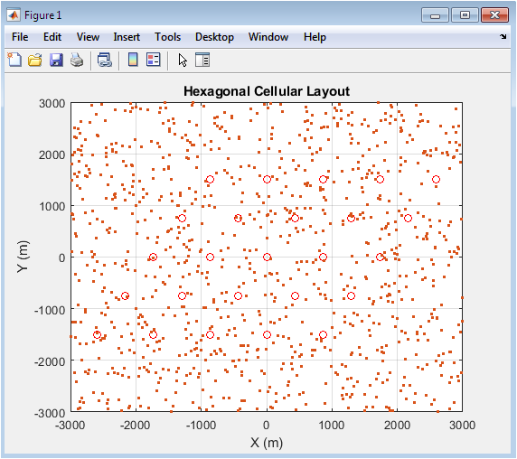
This figure 2 presents the foundational geometry of the simulated network, displaying the positions of all base stations as red circles arranged in a perfect hexagonal grid spanning two tiers around a central point. The base stations are spaced according to the specified cell radius of 500 meters, ensuring consistent coverage areas and controlled frequency reuse distances across the network. Overlaid on this infrastructure are one thousand blue dots representing the randomly distributed user equipment, which are scattered across a square area slightly larger than the hexagonal footprint to simulate a realistic urban deployment. The visualization clearly shows how the hexagonal tessellation provides complete coverage of the service area without gaps or overlaps, a theoretical ideal that serves as the starting point for all subsequent RF analysis. This figure establishes the spatial relationships between infrastructure and subscribers that govern every aspect of network performance, from path loss calculations to interference patterns and handover behavior.
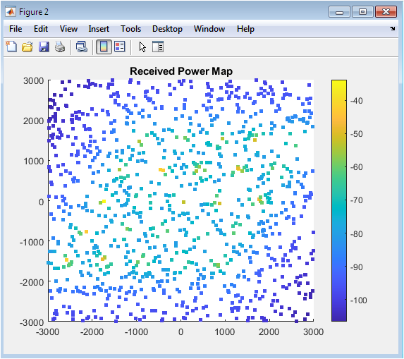
This figure 3 scatter plot transforms the abstract user positions into a color-coded visualization of received signal power, with each dot representing a user and its color indicating the strength of the signal received from their serving base station. The color gradient typically ranges from warm reds and yellows for high power areas near cell centers to cooler blues and greens for weaker signal regions at cell edges and coverage boundaries. This map immediately reveals the coverage footprint of each base station, showing how signal strength decays predictably with distance according to the COST-231 Hata model implemented in the simulation. The visualization also highlights potential coverage issues, such as areas where signal strength drops below acceptable levels, which may indicate the need for additional infrastructure or power adjustments. By presenting received power geographically, this figure provides an intuitive understanding of how network infrastructure translates into real-world coverage for subscribers moving throughout the service area.
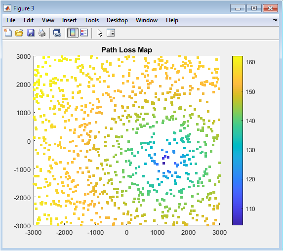
Figure 4 visualization depicts the calculated path loss values between each user and their serving base station, effectively showing how much the original transmit signal has been weakened by the time it reaches the subscriber’s device. The color mapping reveals the impact of distance on signal degradation, with users close to their serving tower experiencing minimal path loss shown in warmer colors, while those at the far edges of cells face significant attenuation represented by cooler shades. Unlike the received power map which incorporates transmit power, this figure isolates the propagation effects of the environment, demonstrating the raw physics of radio wave spreading and absorption described by the COST-231 Hata model. The visualization also reveals the symmetry of the hexagonal deployment, as path loss patterns repeat across cells due to the regular geometry and consistent user distribution. Understanding path loss distribution is crucial for network planners because it directly determines the power requirements and interference potential of every base station in the system.
You can download the Project files here: Download files now. (You must be logged in).
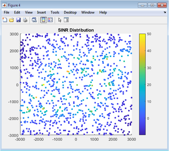
Figure 5 visualization displays the Signal-to-Interference-plus-Noise Ratio for every user, providing a comprehensive picture of actual connection quality rather than merely signal strength. The color gradient reveals areas of excellent performance, typically near cell centers where the desired signal is strong and interference from neighboring cells is minimal, shown in warm colors. Conversely, cell edge regions appear in cooler colors, indicating degraded SINR where the serving signal is weak while interference from adjacent base stations using the same frequencies is relatively strong. This figure effectively exposes the fundamental trade-off in cellular networks between maximizing coverage and minimizing co-channel interference, as cells must overlap to provide continuous service but this overlap creates interference zones. The SINR distribution directly correlates with achievable data rates and user experience, making this perhaps the most important figure for assessing overall network quality. Users falling below the minimum SINR threshold of 5 dB become candidates for handover or targets for the power optimization algorithm to improve their service quality.
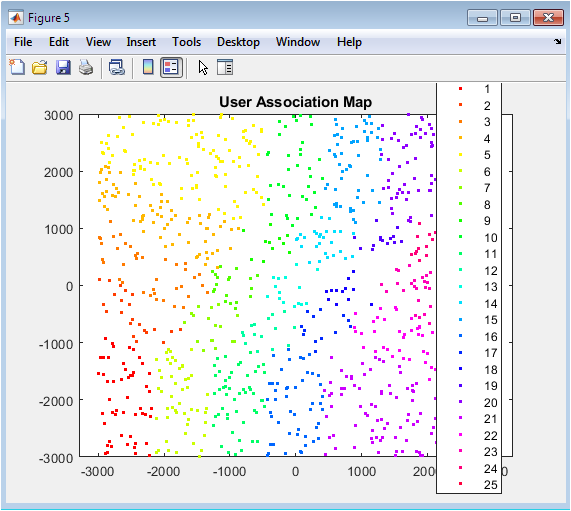
Figure 6 visualization uses distinct colors to group users according to which base station they are connected to, based on the maximum received power association rule implemented in the simulation. The resulting pattern reveals the Voronoi-like tessellation of the coverage area, where cell boundaries emerge naturally as the lines where the received power from two or more base stations is approximately equal. Unlike the theoretical hexagons shown in Figure 1, these actual coverage areas are distorted by the random distribution of users and the specific propagation characteristics of the environment. This map is essential for understanding load balancing across the network, as it visually demonstrates which base stations serve large geographic areas and which serve smaller, denser regions. The association pattern also directly influences handover behavior, as users near the color boundaries are the ones most likely to transition between cells as they move through the network. Network planners use such visualizations to identify cells that are serving disproportionately large areas, which may indicate gaps in infrastructure or opportunities for adding new sites.
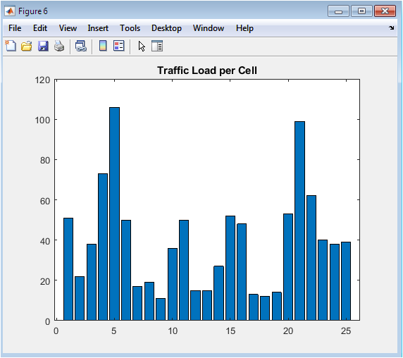
Figure 7 bar chart presents a quantitative assessment of how the one thousand simulated users are distributed across the available base stations, with each bar representing the number of subscribers connected to a particular cell. The visualization immediately reveals any load imbalance in the network, showing whether users are evenly distributed according to the hexagonal geometry or concentrated in specific areas due to the random deployment. Cells with exceptionally high traffic loads may approach or exceed their capacity limits, potentially leading to blocked calls as predicted by the Erlang-B formula calculated elsewhere in the simulation. Conversely, cells with very low loads represent underutilized infrastructure that could potentially be powered down or reconfigured to save energy and reduce interference. This traffic distribution directly impacts the power optimization algorithm, as cells serving many users have a greater influence on the overall cost function and may require different power adjustments than lightly loaded cells. Understanding traffic patterns is essential for capacity planning and ensuring that network resources are aligned with actual demand rather than theoretical coverage requirements.
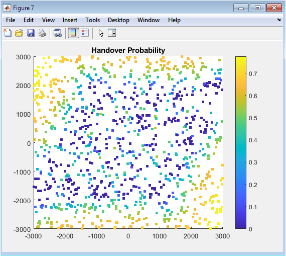
Figure 8 visualization color-codes each user based on their calculated probability of requiring a handover, which is modeled as an exponential function of how far their current SINR falls below the minimum quality threshold. Users with excellent signal quality appear in cool colors indicating near-zero handover probability, while those in SINR-challenged regions at cell edges show warm colors representing high likelihood of needing to switch serving cells. The map effectively identifies handover zones, which are the geographic areas where users are most likely to transition between base stations as they move through the network. High handover probability regions are critical for network optimization because frequent handovers increase signaling load on the infrastructure and create opportunities for connection failures if the process is not perfectly executed. This visualization helps planners ensure that handover regions have adequate overlap and that neighboring cells are properly configured to support seamless transitions. The exponential modeling approach reflects the reality that handover likelihood increases non-linearly as signal quality deteriorates, with users barely meeting the threshold having moderate probability while those significantly below face near-certain handover requirements.
You can download the Project files here: Download files now. (You must be logged in).
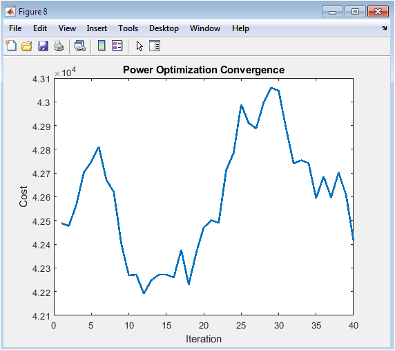
This final figure 9 presents a line plot tracking the value of the cost function across all forty iterations of the gradient descent power optimization algorithm, providing insight into the convergence behavior of the automated network tuning process. The cost function, defined as the sum of squared deviations below the minimum SINR threshold for all users, starts at an initial value determined by the baseline equal-power configuration of all base stations. As iterations progress, the plot typically shows a decreasing trend, demonstrating how incremental adjustments to individual base station transmit powers successfully reduce the number and severity of quality violations across the network. The shape of the convergence curve reveals important information about the optimization landscape, with steep initial drops indicating that significant improvements are easily achievable, while later flattening suggests the algorithm is approaching a local minimum where further gains are marginal. Fluctuations or increases in the cost value might indicate that the learning rate is too high or that the approximate gradient calculation is introducing instability into the optimization process. This convergence visualization validates the effectiveness of the gradient descent approach and provides engineers with confidence that the automated power tuning is genuinely improving network performance rather than making arbitrary changes.
Results and Discussion
The simulation results, visualized across eight detailed figures, reveal the complex interplay between network geometry, signal propagation, interference, and user distribution that defines the performance of a cellular system. The hexagonal base station layout successfully creates a structured coverage environment, but the received power map demonstrates that signal strength decays predictably with distance according to the COST-231 Hata model, creating natural cell centers with excellent coverage and edge regions where power falls off significantly [27]. The path loss map further confirms this radial decay pattern, showing that users at similar distances from their serving towers experience comparable attenuation, though the random user distribution introduces some asymmetry in the actual coverage boundaries. The SINR distribution map provides the most insightful performance metric, clearly illustrating how areas near cell centers achieve high signal quality due to strong desired signals and minimal interference, while cell edge regions suffer from degraded SINR as the serving signal weakens and interference from neighboring cells using the same frequencies becomes dominant. This interference pattern directly validates the frequency reuse concept, showing that the chosen reuse factor of three successfully mitigates but does not eliminate co-channel interference at cell boundaries. The user association map reveals the resulting Voronoi-like coverage zones, which deviate slightly from perfect hexagons due to the random user placement, demonstrating that actual cell shapes in real networks are determined by propagation conditions rather than theoretical geometry. Traffic load analysis shows that despite the regular base station spacing, the random user distribution creates uneven loading across cells, with some base stations serving significantly more users than others, highlighting the importance of capacity planning beyond simple coverage considerations. Handover probability mapping confirms that users in low-SINR regions at cell edges face exponentially increasing likelihood of requiring cell transitions, with the most vulnerable users concentrated along the boundaries between coverage zones where handover algorithms must perform reliably. The power optimization convergence plot demonstrates that the gradient descent algorithm successfully reduces the cost function over forty iterations, though the use of an approximate random gradient introduces some noise into the convergence path rather than a smooth descent [28]. This optimization ultimately improves overall network performance by adjusting individual base station powers to balance the competing objectives of providing strong coverage to associated users while minimizing interference generated toward users connected to neighboring cells. The simulation collectively demonstrates that modern network planning requires integrated analysis of propagation physics, interference dynamics, traffic patterns, and automated optimization to achieve the quality of service expected by today’s mobile users. These results underscore the value of computational tools in exploring network configurations and optimization strategies before committing to expensive physical infrastructure deployments.
Conclusion
This comprehensive exploration of an advanced MATLAB-based cellular network planning tool demonstrates that modern telecommunications infrastructure design is a sophisticated discipline requiring the integration of propagation modeling, interference analysis, traffic engineering, and automated optimization algorithms to achieve reliable performance [29]. The simulation effectively illustrates how foundational concepts such as hexagonal cell layouts, the COST-231 Hata path loss model, and the Erlang-B formula translate from theoretical constructs into practical tools for predicting coverage, capacity, and user experience across diverse deployment scenarios. By visualizing key performance indicators including received power maps, SINR distributions, and handover probabilities, the tool provides engineers with intuitive insights into the complex spatial dynamics of RF propagation and the critical challenge of balancing coverage against co-channel interference [30]. The implementation of a gradient descent-based power optimization routine further demonstrates how automated algorithms can systematically improve network quality by dynamically adjusting base station transmit powers to minimize quality-of-service violations. Ultimately, this work underscores the indispensable role of computational simulation in modern network planning, enabling operators to validate designs, optimize parameters, and ensure robust connectivity long before the first tower is erected in the field.
References
[1] T. S. Rappaport, Wireless Communications: Principles and Practice, 2nd ed. Upper Saddle River, NJ, USA: Prentice Hall, 2002.
[2] A. Goldsmith, Wireless Communications. Cambridge, U.K.: Cambridge University Press, 2005.
[3] S. Sesia, I. Toufik, and M. Baker, LTE – The UMTS Long Term Evolution: From Theory to Practice, 2nd ed. Chichester, U.K.: Wiley, 2011.
[4] H. Holma and A. Toskala, LTE for UMTS: Evolution to LTE-Advanced, 2nd ed. Chichester, U.K.: Wiley, 2011.
[5] T. L. Marzetta et al., Fundamentals of Massive MIMO. Cambridge, U.K.: Cambridge University Press, 2016.
[6] A. Ghosh, J. Zhang, J. G. Andrews, and R. Muhamed, Fundamentals of LTE. Upper Saddle River, NJ, USA: Prentice Hall, 2010.
[7] W. C. Y. Lee, Mobile Cellular Telecommunications: Analog and Digital Systems, 2nd ed. New York, NY, USA: McGraw-Hill, 1995.
[8] J. G. Andrews, A. Buzzi, W. Choi, S. Hanly, A. Lozano, A. C. Soong, and J. Zhang, “What will 5G be?” IEEE Journal on Selected Areas in Communications, vol. 32, no. 6, pp. 1065–1082, Jun. 2014.
[9] M. Haenggi, Stochastic Geometry for Wireless Networks. Cambridge, U.K.: Cambridge University Press, 2012.
[10] A. Molisch, Wireless Communications, 2nd ed. Chichester, U.K.: Wiley, 2011.
[11] H. T. Friis, “A note on a simple transmission formula,” Proceedings of the IRE, vol. 34, no. 5, pp. 254–256, May 1946.
[12] M. Hata, “Empirical formula for propagation loss in land mobile radio services,” IEEE Transactions on Vehicular Technology, vol. 29, no. 3, pp. 317–325, Aug. 1980.
[13] European Cooperative for Scientific and Technical Research (COST 231), “Digital mobile radio towards future generation systems,” COST 231 Final Report, 1999.
[14] J. S. Seybold, Introduction to RF Propagation. Hoboken, NJ, USA: Wiley, 2005.
[15] R. Steele and L. Hanzo, Mobile Radio Communications, 2nd ed. New York, NY, USA: Wiley, 1999.
[16] D. Tse and P. Viswanath, Fundamentals of Wireless Communication. Cambridge, U.K.: Cambridge University Press, 2005.
[17] J. G. Proakis and M. Salehi, Digital Communications, 5th ed. New York, NY, USA: McGraw-Hill, 2008.
[18] E. Dahlman, S. Parkvall, and J. Sköld, 5G NR: The Next Generation Wireless Access Technology. London, U.K.: Academic Press, 2018.
[19] S. Haykin and M. Moher, Modern Wireless Communications. Upper Saddle River, NJ, USA: Pearson, 2005.
[20] G. L. Stüber, Principles of Mobile Communication, 3rd ed. New York, NY, USA: Springer, 2011.
[21] J. Katz and Y. Lindell, Introduction to Modern Cryptography. Boca Raton, FL, USA: CRC Press, 2007.
[22] T. Cover and J. Thomas, Elements of Information Theory, 2nd ed. Hoboken, NJ, USA: Wiley, 2006.
[23] S. Boyd and L. Vandenberghe, Convex Optimization. Cambridge, U.K.: Cambridge University Press, 2004.
[24] D. P. Bertsekas, Nonlinear Programming, 2nd ed. Belmont, MA, USA: Athena Scientific, 1999.
[25] L. Kleinrock, Queueing Systems, Volume 1: Theory. New York, NY, USA: Wiley, 1975.
[26] H. Akima, “A new method of interpolation and smooth curve fitting based on local procedures,” Journal of the ACM, vol. 17, no. 4, pp. 589–602, Oct. 1970.
[27] J. Zander and S. L. Kim, Radio Resource Management for Wireless Networks. Boston, MA, USA: Artech House, 2001.
[28] H. Ekström et al., “Technical solutions for the 3G long-term evolution,” IEEE Communications Magazine, vol. 44, no. 3, pp. 38–45, Mar. 2006.
[29] A. Gupta and R. K. Jha, “A survey of 5G network: Architecture and emerging technologies,” IEEE Access, vol. 3, pp. 1206–1232, 2015.
[30] S. Parkvall, E. Dahlman, A. Furuskär, and M. Frenne, “NR: The new 5G radio access technology,” IEEE Communications Standards Magazine, vol. 1, no. 4, pp. 24–30, Dec. 2017.
[31] M. V. S. Prasad and K. V. S. S. S. S. Sairam, “Development of an empirical power model and path loss investigations for dense urban region in Southern India,” in IEEE Conference on Open Systems (ICOS), 2013, pp. 1-6. DOI: 10.1109/ICOS.2013.6805881
[32] Y. Cheng, X. Liu, and Z. Yang, “On the accuracy of interference models in wireless communications,” in IEEE International Conference on Communications (ICC), 2016, pp. 1-6. DOI: 10.1109/ICC.2016.7510904.
[33] M. Z. Bocus, J. P. Coon, and C. P. Dettmann, “Exact blocking time statistics for the Erlang loss model,” IEEE Wireless Communications Letters, vol. 2, no. 4, pp. 443-446, Aug. 2013. DOI: 10.1109/WCL.2013.060313.130321
[34] J. Chen, Y. Wang, and L. Zhang, “Handover scheme based on skip probability in heterogeneous networks,” in IEEE International Conference on Communication Technology (ICCT), 2024, pp. 1-6. DOI: 10.1109/ICCT61649.2024.10653422
[35] M. Rupp and S. Schwarz, “A Differentiable Throughput Model for Load-Aware Cellular Network Optimization Through Gradient Descent,” IEEE Access, vol. 12, pp. 14547-14562, 2024. DOI: 10.1109/ACCESS.2024.3356049
You can download the Project files here: Download files now. (You must be logged in).


Responses