

Hexapod CPG Gait Generator: Tripod, Ripple and Wave
Simulate six coupled Hopf oscillators, blend tripod–ripple–wave gaits, and animate reachable three-joint leg commands. Inspect phase tracking, footfall timing and joint speed.

A central pattern generator turns a few control settings into coordinated leg rhythms. This hexapod CPG gait generator lets engineers, students and robotics builders explore how six coupled nonlinear Hopf oscillators synchronize, recover from an initial phase disturbance and switch between tripod, ripple and wave gaits. It integrates both oscillator amplitudes and phases, then generates foot paths and solves the coxa, femur and tibia commands for all six legs.
Choose the start, middle and final gaits. The default program runs tripod first, blends into ripple, then blends into wave. Set the same gait in all three fields to study steady synchronization. The first transition starts at the specified time; the second starts after one transition duration and the middle-gait dwell. The simulation continues for three nominal strides after the second transition finishes.
Stride frequency sets the common oscillator frequency. Coupling gain controls how quickly relative phases track their targets. Radial convergence controls recovery toward the Hopf limit cycle, while initial radius controls the starting stroke and lift. The phase disturbance deliberately starts different legs away from their targets. Try reducing coupling or shortening the transition to see phase tracking deteriorate. Very fast transitions can reverse an oscillator temporarily; the calculator reports this behavior.
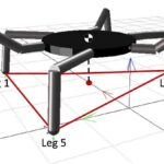
Press play or scrub animation time to inspect the legs. Blue phase hands on the body represent the six coupled oscillators. Teal legs are in commanded stance and amber legs are in swing. LF, LM and LR mean left front, middle and rear; RF, RM and RR are their right-side counterparts. The footfall chart uses the same colors, dashed lines mark transition starts, and its blue cursor follows the animation. Red markers identify intervals with zero commanded stance, including gaps narrower than one chart pixel.
Tripod alternates two groups of three legs. Ripple uses six staggered phases with two overlapping swings and a stance duty factor of 2/3. Wave uses six staggered phases with one swing and a duty factor of 5/6. The exact leg orders are defined in the method because ripple terminology varies between robot projects. Coupling targets and duty factors change through a quintic ramp, while the oscillator states continue without phase resets.
Enter the three link lengths, outward foot reach, hip height, stroke and lift to match a proposed leg. The table shows simultaneous joint commands; the LF chart shows their history and the peak LF command speed helps compare timing choices. Joint angles use geometric zeros, so hardware needs servo offsets and mirrored sign conventions. Reachability conditions reject paths too close to full extension or folding.
This tool covers rhythm generation and kinematic commands. It does not calculate contact forces, body balance, motor torque, actuator saturation, terrain response or collisions. A smooth CPG gait transition can still produce an unsuitable support pattern. The animation holds an illustrative chassis stationary, and its commanded stance flags are not contact measurements or a prediction of walking speed.
How it is calculated
The engine integrates all 12 Cartesian states of six nonlinear Hopf oscillators in a common rotating frame. With , unit target radius and node phase targets :
This is rotated diffusive coupling of the full Hopf states. Coupling acts on both radius and phase, so transient loss of coordination can reduce amplitude. The sum is evaluated in the node-target frame through its mean Cartesian vector, an exact algebraic rearrangement of all six pair contributions. The common rotation is removed by the exact transformation before integration and restored afterward. The nonlinear Cartesian coupling and amplitude dynamics remain in the ODE. The Hopf foundation follows Ijspeert (2008); Bai et al. (2019), Eqs. 13–18, motivate the six-node oscillator network. The normalized diffusive coupling and three-link kinematics here are explicit design choices, not a reproduction of their curved-leg controller.
The phase targets are negative touchdown lags in the order LF, LM, LR, RF, RM, RR. Tripod uses lags [0, 1/2, 0, 1/2, 0, 1/2] cycles. Ripple uses [0, 1/3, 2/3, 1/2, 5/6, 1/6]; wave uses [0, 1/6, 1/3, 1/2, 2/3, 5/6]. These explicit sequence choices define this generator. Stance duties are 1/2, 2/3 and 5/6, respectively (Mrva 2014, printed p. 8; Bai et al., pp. 4–5). Ripple here has two overlapping swings, unlike the three-pair tetrapod convention.
Each node's shortest phase change is blended using , with clamped to 0…1. Pairwise targets remain consistent because they are always differences of node targets. Duty factor is blended by the same ramp. Oscillator states continue through both transitions without resets.
For , stance is . Stance moves the foot from +stroke/2 to −stroke/2 using ; swing returns it using . Lift is during swing. Stroke and lift are multiplied by . Both foot paths have continuous position, velocity and acceleration at lift-off and touchdown. Closed-form coxa yaw and a planar two-link inverse solve give femur and tibia angles. A forward-kinematic closure property verifies that mapping.
Touchdown events satisfy and lift-off events satisfy , where and is an integer. Crossings are located separately for each leg using the same continuous linear phase interpolation as the animation and the exact quintic duty schedule. Intervals are split at ramp boundaries and at stationary points of before bracketing roots, including during reversals. Touchdown roots are linear solves; lift-off roots use bisection. Events within 10 ns are coalesced to suppress simultaneous-event roundoff. All six stance flags are evaluated between successive events. The minimum and footfall drawing use this shared event partition; final-cycle averages weight interval durations. Red chart markers identify intervals with zero commanded stance.
Adaptive Dormand–Prince integration uses relative tolerance 10⁻⁶. The saved mesh targets at least 100 samples/s and 160 samples per nominal stride, capped at 6,001 saved times. Relative phase RMS compares each of the five other legs with LF after subtracting its scheduled lag. Joint speeds use central differences on that mesh.
Assumptions
Identical intrinsic frequencies; reciprocal all-to-all coupling normalized by six; initial radii in the unit disk; no sensory feedback. The initial disturbance is a fixed unequal phase pattern scaled by the disturbance input. Three nominal strides are retained after the second ramp.
Each leg has an outward coxa followed by femur and tibia hinges in one vertical plane. Coxa zero points outward; positive yaw is forward on both sides. Femur zero is horizontal outward, positive upward. Tibia zero is straight extension and flexion is negative. Mirror these signs and add servo zero offsets for actual hardware.
The stationary chassis and hip spacing are illustrative. The drawn links and foot trajectories use the entered lengths; chassis half-width is 0.4 times foot reach and front/rear hip spacing is 0.7 times foot reach. The diagram uses an oblique projection.
Where it applies
This is an open-loop rhythm and joint-command generator. Commanded stance is a timing state, not measured contact. Smooth phase transitions do not establish balance: there is no body dynamics, support-polygon margin, contact force, traction, terrain compliance, collision detection, servo saturation, torque, power or load model. It does not predict walking speed; the quintic stance path does not enforce constant ground speed.
All commanded feet must stay more than 1 mm from full folding and full extension. Conservative reach bounds cover the entire stroke and lift. Inverse-trigonometric arguments are clamped only for numerical robustness; invalid geometries are blocked by conditions. Phase reversal is reported when a sampled phase speed becomes nonpositive; lengthen the transition or raise the stride frequency.
Cartesian states give radii and unwrapped phases. The animation linearly interpolates these saved radii and unwrapped phases, then recomputes the foot path and inverse kinematics. Saved output is capped at 6,001 times to keep long programs interactive. Event roots resolve contact crossings within the interpolated phase histories, rather than assigning an entire sample interval one contact state. Event timing accuracy is limited by the ODE solution and phase interpolation; the 10 ns grouping tolerance is not a claim of physical timing accuracy. At the output cap, rapid phase curvature can shift event times and sampled joint-speed peaks can be underestimated, especially during short wave-gait swings. The adaptive ODE tolerance is unchanged. The reported final error is at the end of the three-stride observation window; weak coupling can require longer to lock. No physical balance or hardware experiment is claimed.
References
- Ijspeert, A. J. (2008). Central pattern generators for locomotion control in animals and robots: A review. Neural Networks 21, 642–653. https://doi.org/10.1016/j.neunet.2008.03.014
- Bai, L., Hu, H., Chen, X., Sun, Y., Ma, C., and Zhong, Y. (2019). CPG-Based Gait Generation of the Curved-Leg Hexapod Robot with Smooth Gait Transition. Sensors 19, 3705. https://doi.org/10.3390/s19173705 (attached full text s4).
- Mrva, J. (2014). Design of Motion Primitives for a Hexapod Walking Robot Operating in a Rough Environment. CTU master's thesis, printed pp. 7–9, 17. https://cyber.felk.cvut.cz/theses/papers/480.pdf
Inputs
| Input | Symbol | Unit | Default |
|---|---|---|---|
| Start gait | g_start | Tripod | |
| Middle gait | g_mid | Ripple | |
| Final gait | g_end | Wave | |
| Stride frequency | f_cpg | Hz | 1 |
| Phase coupling gain Mean coupling to all six oscillators; larger values track the phase targets faster. | K_c | 1/s | 6 |
| Radial convergence rate | alpha_h | 1/s | 4 |
| Initial oscillator radius | r_init | 0.6 | |
| Initial phase disturbance Scales a fixed unequal disturbance across the six legs. | phase_seed | deg | 15 |
| First transition starts | t_switch | s | 3 |
| Transition duration | T_morph | s | 2 |
| Middle gait dwell | T_hold | s | 2 |
| Coxa length | L_c | mm | 35 |
| Femur length | L_f | mm | 75 |
| Tibia length | L_t | mm | 110 |
| Outward foot reach Lateral distance from the coxa axis to the nominal foot line. | R_foot | mm | 130 |
| Hip height | H_body | mm | 100 |
| Fore–aft stroke | S_step | mm | 70 |
| Swing lift | H_lift | mm | 25 |
| Animation time | t_play | s | 9.68 |
Results
With the default inputs above, the calc gives:
| Result | Value |
|---|---|
| Uncoupled stride period | 1 s |
| Final relative phase RMS error | 0 deg |
| Peak relative phase RMS error | 12.72 deg |
| Minimum commanded stance legs | 0 |
| Peak LF joint command speed | 394.4 deg/s |
Checked against sources
Each case below was calculated by this calc and agrees with the value from its source (within the tolerance where one is shown).
Published tripod timing
Source: Bai et al. 2019, Sensors 19, 3705, pp. 4–5, duty 0.5 and three stance legs. A steady-gait timing benchmark, not a reproduction of their curved-leg robot experiments. Unit Hopf radius follows their Eq. 13 with R = 1.
Inputs: Middle gait = Tripod; Final gait = Tripod; Initial phase disturbance = 0 deg; the others as above.
| Result | Source | This calc |
|---|---|---|
| Mean stance count in the final cycle | 3 ± 0.02 | 3 |
| Measured LF stance duty in the final cycle | 0.5 ± 0.01 | 0.5 |
| Final oscillator radius | 1 | 1 |
| Minimum commanded stance legs | 3 | 3 |
Published ripple timing
Source: Mrva 2014, printed p. 8 (attached p. 14): ripple has two legs in transfer at different times and a 2/3 support duty. This checks steady timing only; leg sequence choices are declared separately.
Inputs: Start gait = Ripple; Final gait = Ripple; Initial phase disturbance = 0 deg; the others as above.
| Result | Source | This calc |
|---|---|---|
| Mean stance count in the final cycle | 4 ± 0.02 | 4 |
| Measured LF stance duty in the final cycle | 0.6667 ± 0.01 | 0.6667 |
| Minimum commanded stance legs | 4 | 4 |
Published wave timing
Source: Bai et al. 2019, pp. 4–5 and Section 3.3: wave duty 5/6, five stance legs and sequential phase spacing 1/6 of 2π = 60°. Steady timing benchmark only.
Inputs: Start gait = Wave; Middle gait = Wave; Initial phase disturbance = 0 deg; the others as above.
| Result | Source | This calc |
|---|---|---|
| Mean stance count in the final cycle | 5 ± 0.02 | 5 |
| Measured LF stance duty in the final cycle | 0.8333 ± 0.01 | 0.8333 |
| Final minimum circular phase gap | 60 deg | 60 deg |
| Minimum commanded stance legs | 5 | 5 |
Startup gap between contact events
Source: Independent review supplied with this calculator task: an independent ODE integration confirms a brief all-six-swing startup interval containing t = 0.429 s at the default oscillator settings. This regression must report both the instantaneous zero count and a zero minimum over the complete run.
Inputs: Animation time = 0.429 s; the others as above.
| Result | Source | This calc |
|---|---|---|
| Minimum commanded stance legs | 0 | 0 |
| Current commanded stance legs | 0 | 0 |





Responses