

2D FDTD Simulator: Yee Grid, TMz Waves and PML Boundary
Animate TMz waves on an 80×80 Yee grid with graded PML or reflecting PEC walls. Calculate the Courant time step, PML conductivity, ideal reflection and residual field energy.

Explore how electromagnetic waves leave a finite computation window with this 2D FDTD simulator. It uses the TMz polarization: the electric field Ez points out of the screen, while Hx and Hy lie in the screen. A soft Gaussian point source launches a circular pulse on a Yee grid. Engineers and students can watch the pulse enter a graded perfectly matched layer, or select a PEC wall to see reflected waves return.
Start with the defaults: 80×80 electric nodes, 10 mm spacing, a Courant safety factor of 0.95, and a 20-cell PML on each side. Press ▶ beside Playback step, or move that slider to inspect a saved frame. Frames are stored every eight steps. The field uses a fixed symmetric blue–red scale, so fading colours indicate decreasing field amplitude. The dashed box marks the inner PML interface; the black cross identifies the source. The colour scale shows Ez divided by the peak source increment, rather than an automatically rescaled image.
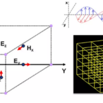
Change the grid spacing to set the physical length scale. The calculator derives the time step from the two-dimensional Courant limit and reports the number of steps needed to cross the longer useful interior side in vacuum. Increasing relative permittivity above one inserts a small lossless rectangular block. Refraction, scattering and slower propagation then appear; the exterior and the PML remain vacuum. The Yee grid calculator schematic explains why the magnetic fields sit half a cell and half a time step away from the electric field.
The PML boundary conditions use matched electric and magnetic losses, sampled at their staggered locations. Thickness, grading order and target amplitude reflection determine the maximum conductivity. The reflection chart holds that conductivity fixed while varying thickness, and compares the selected order with the next order. It is a continuum normal-incidence estimate of a round trip to the outer wall. It is not a measured reflection coefficient of the discrete simulation. Changing the design thickness recalculates conductivity to meet the chosen target.
The energy chart and final residual describe the actual simulated fields outside the PML. Energy is sampled every four steps and normalized to its peak during the run. A nonzero remainder can include a long pulse tail, dielectric scattering, numerical dispersion and discrete-PML reflections. Extend the run to inspect its decay.
For readers looking for 2D FDTD MATLAB implementations, this browser tool exposes the same leapfrog equations without requiring a local MATLAB installation. It is limited to two-dimensional, linear, nonmagnetic, nondispersive media. It does not calculate antenna impedance, radiation patterns, three-dimensional modes or certified absorber performance. The article’s 200×200 grid is too heavy for this interactive browser calculation; the smaller fixed grid keeps recomputation and animation practical.
How it is calculated
The original implementation here follows the TMz Yee staggering explained in EMPossible, 2D FDTD formulation (attached s3), and McMaster ECE757 (s2, pp. 1–10). With vacuum outside the block, the fastest speed is , and
The spatial grid has 80×80 Ez nodes; outer PEC nodes are 79 cell widths apart. The source is at cell coordinates (39.5,39.5), shared equally between the four nearest electric nodes. Hx sits at (x,y+Δy/2), Hy at (x+Δx/2,y), and H is advanced half a time step ahead of E.
For split-field PML, write . The differential equations are
In the vacuum PML, . Centering the loss term gives , and . Conductivity is sampled at the actual E and H locations; x and y losses both act in the corners. Inside the dielectric, losses vanish and electric curl increments are divided by εr. The solver stores Ez/Edrive and η₀H/Edrive. This is Berenger split-field PML, not a uniform lossy sponge and not CPML.
For distance into a layer, . At normal incidence, a PEC-terminated continuum layer has round-trip amplitude
Therefore , separately for and . The thickness chart holds the current x-normal σmax fixed and compares m with m+1. Amplitude dB uses 20 log₁₀; energy dB uses 10 log₁₀.
Source correction: Wang et al., arXiv:2509.20801, attached s5 p. 4 Eq. (13), prints ln[R(0)] with a positive prefactor. That would give negative loss for 0<R<1; the attenuation integral requires −ln R = ln(1/R). Its Eqs. (11)–(12) also include /Δ. Here σmax is explicitly in S/m and is applied only once, without an additional division by cell size. Corbino, arXiv:2603.19056v2, s6 p. 8 Eq. (29), supplies a separate conductivity-rule cross-check; the paper’s mimetic damping code is not copied or treated as a split-field benchmark.
At every step the soft increment is added equally to the two electric splits at the source. It stops after n=8τs. The setup is symmetric about y = 39.5. The solver advances the lower half-domain with even Ez and Hy and odd Hx. For vacuum it also uses x symmetry, advancing one quarter. The block breaks x symmetry, so that case advances the full width. Mirroring reconstructs the full 80×80 field exactly for the specified source and geometry. Energy sums are scaled to represent the full domain. Colour frames are precomputed every eight steps; energy is sampled every four steps. For the energy diagnostic, average E at n and n−1 and combine it with H at n−½, using per unit z length. Only nodes and edges between the inner PML interfaces are summed; in PEC mode the entire domain is used. This simple quadrature is a diagnostic, not an exact discrete conserved energy. The residual is final sampled energy divided by the largest sampled energy of the same run.
Independent check of absorption
Boito et al. (2020), attached s10 p. 6 Eqs. (43)–(44), provide the retarded 2D scalar-wave Green function. With normalization , its kernel is
It is applied to the TMz scalar wave equation here; the reference uses no finite boundary or PML equations. Each soft increment is represented as constant Ampere drive during . Its time derivative gives two impulses. After the pulse has passed, their exact convolution is
where and the four source nodes are (39,39), (40,39), (39,40), (40,40). This evaluates a published analytical solution for the tool’s specified excitation; the numbers are not claimed as a published numerical table.
The frozen benchmark uses vacuum, Δx=Δy=10 mm, safety 0.95, τs=8, 20-cell cubic PML and target R=10⁻⁶. At probe nodes (39,39) and (49,39), the exact normalized fields are respectively −0.000304718749 and −0.000310405656 at step 160, and −0.000176765461 and −0.000178660114 at step 200. Both times allow an undamped return from the outer wall, so the comparison tests absorption. Each case allows 2% relative error for the finite grid and discrete boundary. A read-only mutation removing both PML loss factors makes these late-field comparisons fail, while leaving the early stencil check intact. This verifies absorption at the benchmark’s accuracy; it does not certify the continuum reflection target as a measured discrete reflection.
Assumptions
TMz only, invariant along z. Fields begin at zero. Vacuum has c₀ = 299792458 m/s and η₀ = 376.730313668 Ω; ε₀ is derived consistently as 1/(η₀c₀). The soft source has a fixed peak increment of 1 V/m, so all displayed energies scale with its square.
The optional block uses constant εr ≥ 1 and μr = 1, occupying electric nodes x = 46…52 and y = 33…46, with cell edges shown on the field image. Setting εr = 1 removes it. There are no material losses, dispersion or nonlinearities. The PML is entirely in vacuum and is backed by a PEC edge.
Reference cases distinguish their scope: the Courant case checks a published convention; the conductivity case is algebraic consistency; and the early scalar-wave case checks the interior stencil before PML arrival. Two additional late-time cases compare the actual absorbing run against an independent analytical unbounded-space Green function. The reference numbers are evaluated from the published exact solution, not copied from a paper’s numerical table. Physical invariants supplement these checks.
Where it applies
Use cell aspect ratios from 0.5 to 2, 4–24 PML cells, grading orders 1–5 and Courant safety factors 0.4–0.99. With a dielectric block, leave at least four vacuum cells before the PML. Simulation length must be a multiple of eight. Playback shows the preceding stored frame (eight-step spacing); colour limits stay fixed at ±0.04 of the source increment and larger values are colour-clipped.
The Gaussian spectrum reaches −20 dB in amplitude at f₂₀ = √ln(10)/(πτ). The reported wavelength resolution uses the highest permittivity and the larger cell size. Ten cells per wavelength is only a screening rule: all results still have directional numerical dispersion, staircased material interfaces and finite-grid PML error. Refine and test convergence in a full solver for quantitative design.
The continuum target is an amplitude ratio, with reflected power R². It predicts attenuation of an ideal normally incident return from the outer wall; it does not include discrete interface mismatch, oblique or grazing waves, the point source’s low-frequency tail, or resonances. More aggressive σmax is not guaranteed to reduce the simulated residual. Energy sampled every four steps can miss a peak and is shown with a −120 dB chart floor. The last diagnostic is at (Nrun−½)Δt. A residual is not a measured reflection coefficient.
The centred source and fixed block are mirror-symmetric in y; arbitrary off-centre geometry is outside this tool. The fixed 80×80 electric-node mesh is intentional. The article’s 200×200 grid is too heavy for this browser’s interactive computation and storage budget. Use a dedicated FDTD package for larger grids, 3D, conductive/dispersive media, CPML, calibrated scattering parameters or radiation quantities.
References
- Raymond C. Rumpf, EMPossible EMP-5304, Formulation of 2D FDTD Without PML; The Perfectly Matched Layer; Implementation of 2D FDTD. Open lecture notes: https://empossible.net/academics/emp5304/
- Mohamed Bakr, McMaster ECE757, 2016, FDTD Part 2, especially pp. 10 and 13 (CFL and TMz PEC). https://www.ece.mcmaster.ca/faculty/bakr/ECE757/FDTD_2_2016.pdf
- J.-P. Berenger, A perfectly matched layer for the absorption of electromagnetic waves, J. Comput. Phys. 114(2), 185–200 (1994). https://doi.org/10.1006/jcph.1994.1159 (cited by DOI; no paywalled full text attached).
- Z. Wang et al., Parallel overlapping-domain decomposition FDFD for large-scale complex nanostructures modeling (2025), §2.2, Eqs. (11)–(13). Sign and dimensional convention discussed in Method. https://arxiv.org/abs/2509.20801
- J. Corbino, Solving Maxwell’s Equations with Mimetic Methods (2026), v2, §§5.1, 6.2. Courant-number and conductivity-rule checks only; different field solver. https://arxiv.org/abs/2603.19056v2
- D. Boito et al., On Maxwell’s electrodynamics in two spatial dimensions, Rev. Bras. Ensino Fis. 42, e20190323 (2020), Eqs. (43)–(44), open-access exact Green function used for late-time absorption benchmarks. https://doi.org/10.1590/1806-9126-RBEF-2019-0323; https://arxiv.org/abs/1809.07368v3
Inputs
| Input | Symbol | Unit | Default |
|---|---|---|---|
| Cell width Δx 80 electric nodes in x. The outer nodes are 79 cell widths apart. | dx | mm | 10 |
| Cell height Δy 80 electric nodes in y. Keep the cell aspect ratio between 0.5 and 2. | dy | mm | 10 |
| Courant safety factor Δt is this fraction of the vacuum 2D Courant limit. The dielectric block only slows the wave. | safety | 0.95 | |
| Block relative permittivity (1 = vacuum) Lossless, nonmagnetic block at x = 46…52 and y = 33…46 cell coordinates. Set 1 for an entirely vacuum domain. | eps_block | 1 | |
| Outer boundary treatment PML ends at an outer PEC wall. PEC mode removes the loss layer; the PML chart still describes the candidate design. | boundary | Graded split-field PML | |
| PML thickness on each side (cells) Included in the 80×80 node domain. A thicker layer reduces the useful interior. | n_pml | 20 | |
| Conductivity grading order m σ(s) = σmax (s/d)ᵐ. The solver samples E and H conductivities at their staggered locations. | m_pml | 3 | |
| Target normal-incidence amplitude reflection Round-trip continuum amplitude estimate, not reflected power and not a guarantee of discrete-grid performance. | R_target | 0.000001 | |
| Gaussian width τ (time steps) Soft point source exp[−((n−4τ)/τ)²], added to Ez. The pulse is switched off after step 8τ. | pulse_steps | 8 | |
| Simulation length (steps) Use a multiple of eight. The 160-step default keeps computation light; extend to 200–280 steps to inspect the late tail. | N_run | 160 | |
| Playback step ▶ Shows the preceding saved colour frame, every eight time steps. Playback reuses precomputed rasters; it never advances the field solver. | n_play | 64 |
Results
With the default inputs above, the calc gives:
| Result | Value |
|---|---|
| Courant-limited time step | 0.02241 ns |
| Steps across longer interior side | 59 |
| Candidate PML σmax in x | 0.36672 S/m |
| Candidate PML σmax in y | 0.36672 S/m |
| Candidate continuum reflection (dB amplitude) | -120 |
| Residual interior energy (%) | 0.0125 |
| Final interior energy per z length | 0 pJ/m |
| Cells per shortest −20 dB wavelength | 11.13 |
Checked against sources
Each case below was calculated by this calc and agrees with the value from its source (within the tolerance where one is shown).
Published Courant number 0.5
Source: Corbino (2026), arXiv:2603.19056v2, attached p. 6, §5.1: published Δt = 0.01/(2c0), Sc = 0.5. This checks the time-step convention only, not the paper's 1D lossy-slab solution. The listed numerical code rounds c0 to 3×10⁸ m/s; this tool uses 299792458 m/s, explaining the 0.069% dt difference.
Inputs: Courant safety factor = 0.7071; the others as above.
| Result | Source | This calc |
|---|---|---|
| Directional Courant number in x | 0.5 | 0.5 |
| Courant-limited time step | 0.01667 ± 2 × 10⁻⁵ ns | 0.01668 ns |
Conductivity-rule consistency (not absorption)
Source: Corbino (2026), arXiv:2603.19056v2, attached p. 8, Eq. (29): σmax = 0.8(p+1)/(ηΔx). The separately stated rule gives 3.2/(120π×0.01) = 0.84882636 S/m for order 3 and Δx = 0.01 m. Choose four PML cells and R = exp(−1.6×4) to compare the target-reflection design with that rule. Physical SI σ is used once, without the extra /Δ appearing in Wang Eq. (11). This is an algebraic consistency check constructed by choosing R to recover Eq. (29); it is not an independently published numerical PML-absorption case.
Inputs: PML thickness on each side (cells) = 4; Target normal-incidence amplitude reflection = 0.001662; the others as above.
| Result | Source | This calc |
|---|---|---|
| Candidate PML σmax in x | 0.8488 ± 0.001 S/m | 0.8494 S/m |
| Candidate PML σmax in y | 0.8488 ± 0.001 S/m | 0.8494 S/m |
Discrete wave-equation field cross-check before PML arrival
Source: Independent second-order scalar wave stencil, derived from the vacuum wave equation, evaluated in numerical-crosscheck.py in the task working folder. With zero initial fields and the same four-node Gaussian current, the recurrence is E[n+1] = 2E[n] − E[n−1] + Cx²δxxE[n] + Cy²δyyE[n] + g[n+1] − g[n]. These expected fields at step 16 come from that separate implementation, not from the Yee solver. The wave's stencil has not yet reached the PML. This is an independent numerical implementation check, not published field data. It does not exercise PML absorption; that is tested by the separate late-time Green-function cases.
Inputs: Simulation length (steps) = 200; the others as above.
| Result | Source | This calc |
|---|---|---|
| Early Ez at the source (step 16) | 0.003764 | 0.003764 |
| Early Ez five cells right of source (step 16) | 7.083 × 10⁻⁵ | 7.083 × 10⁻⁵ |
Unbounded Green-function tail after PML interaction — step 160
Source: Boito et al. (2020), DOI 10.1590/1806-9126-RBEF-2019-0323, attached s10 p. 6 Eqs. (43)–(44). Independent unbounded-space analytical reference evaluated in late-green-benchmark.py; no Yee/PML solver supplies the expected numbers. These are evaluated exact-solution values, not a table published in the paper. Method gives the normalized convolution. Vacuum; 80×80 E nodes indexed 0…79; Δx=Δy=10 mm; safety=0.95. Soft Gaussian g[k]=exp[−((k−32)/8)²], k=1…64, shared equally by nodes (39,39),(40,39),(39,40),(40,40). Each increment is constant Ampere drive g[k]/Δt over [(k−1)Δt,kΔt]. Finite solver: 20-cell cubic PML, target R=10⁻⁶, PEC-backed. Compare normalized Ez at (39,39) and (49,39) at the specified final step, after an undamped outer-wall return could arrive. Absolute tolerances equal 2% of each exact value, allowing finite-grid and discrete-boundary error. This tests absorption, not a certified −120 dB discrete reflection.
Inputs: the default inputs above.
| Result | Source | This calc |
|---|---|---|
| Final normalized Ez at source node (39,39) | -3.047 × 10⁻⁴ ± 6.094 × 10⁻⁶ | -3.046 × 10⁻⁴ |
| Final normalized Ez at probe node (49,39) | -3.104 × 10⁻⁴ ± 6.208 × 10⁻⁶ | -3.104 × 10⁻⁴ |
Unbounded Green-function tail after PML interaction — step 200
Source: Boito et al. (2020), DOI 10.1590/1806-9126-RBEF-2019-0323, attached s10 p. 6 Eqs. (43)–(44). Independent unbounded-space analytical reference evaluated in late-green-benchmark.py; no Yee/PML solver supplies the expected numbers. These are evaluated exact-solution values, not a table published in the paper. Method gives the normalized convolution. Vacuum; 80×80 E nodes indexed 0…79; Δx=Δy=10 mm; safety=0.95. Soft Gaussian g[k]=exp[−((k−32)/8)²], k=1…64, shared equally by nodes (39,39),(40,39),(39,40),(40,40). Each increment is constant Ampere drive g[k]/Δt over [(k−1)Δt,kΔt]. Finite solver: 20-cell cubic PML, target R=10⁻⁶, PEC-backed. Compare normalized Ez at (39,39) and (49,39) at the specified final step, after an undamped outer-wall return could arrive. Absolute tolerances equal 2% of each exact value, allowing finite-grid and discrete-boundary error. This tests absorption, not a certified −120 dB discrete reflection.
Inputs: Simulation length (steps) = 200; the others as above.
| Result | Source | This calc |
|---|---|---|
| Final normalized Ez at source node (39,39) | -1.768 × 10⁻⁴ ± 3.535 × 10⁻⁶ | -1.768 × 10⁻⁴ |
| Final normalized Ez at probe node (49,39) | -1.787 × 10⁻⁴ ± 3.573 × 10⁻⁶ | -1.786 × 10⁻⁴ |
Related Resources
Related articles
Related courses

IEC Electrical Schematics and Industrial Control Panels
5
Original price was: 42 €.21 €Current price is: 21 €.

Basic Electrical Controls & Diagram Reading
7
Original price was: 32 €.18 €Current price is: 18 €.

Modeling Electrical Motor Faults with FEM Simulation using ANSYS MAXWELL
3
Original price was: 50 €.15 €Current price is: 15 €.









Responses