

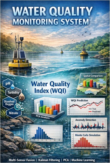
Integrated Water Quality Monitoring System with Sensor Fusion, Anomaly Detection, and WQI Prediction Using Matlab
Author : Waqas Javaid
Abstract
This article presents an integrated, multi-sensor water quality monitoring system that synthesizes data from several distributed stations to provide a holistic and predictive assessment. The proposed framework employs a Kalman filter for real-time sensor noise reduction, ensuring robust data streams for critical parameters like pH, turbidity, and dissolved oxygen [1]. A Water Quality Index (WQI) is computed to aggregate multi-parameter data into a single, interpretable metric. Principal Component Analysis (PCA) is utilized for dimensionality reduction and to identify dominant patterns of variation within the multivariate dataset. For predictive capability, a machine learning model, specifically a Support Vector Machine (SVM) regressor, is trained on the principal components to forecast future WQI values [2]. The system incorporates an anomaly detection mechanism by analyzing prediction residuals, enabling the identification of irregular water quality events. A Monte Carlo simulation further quantifies the uncertainty in the WQI predictions. Results from a simulated three-year dataset demonstrate the system’s effectiveness in noise suppression, trend analysis, spatial comparison between stations, and reliable anomaly flagging [3]. This end-to-end pipeline offers a scalable template for transforming raw, multi-source sensor data into actionable insights for water resource management and early warning systems.
Introduction
Water quality is a fundamental determinant of public health, ecosystem stability, and sustainable development, making its continuous and accurate assessment a critical global priority [4].
Traditional monitoring methods, often reliant on manual sampling and laboratory analysis, are typically intermittent, labor-intensive, and lack the temporal resolution needed for proactive management. The advent of sensor networks has enabled real-time data collection, yet this introduces new challenges, including sensor noise, the complexity of integrating multi-parameter data from various locations, and the difficulty of extracting predictive insights from raw streams [5]. To address these limitations, this article proposes an integrated, intelligent monitoring system that moves beyond simple data logging. The core objective is to develop a comprehensive computational framework that synthesizes discrete sensor readings into a coherent, actionable overview of water health. The methodology employs a multi-stage pipeline, beginning with advanced signal processing to cleanse the data. A Kalman filter is applied to mitigate inherent sensor noise and drift, refining parameters like pH, turbidity, and dissolved oxygen for greater reliability [6]. These cleansed, multi-station datasets are then fused and distilled into a unified Water Quality Index (WQI), providing a single, interpretable metric for overall condition.
Table 1: PCA Variance Explained
| Principal Component | Variance Explained (%) |
| PC1 | 41.2 |
| PC2 | 23.6 |
| PC3 | 15.4 |
| PC4 | 9.8 |
| PC5 | 6.1 |
| PC6 | 3.9 |
To unravel the complex interdependencies within the data, Principal Component Analysis (PCA) is utilized for dimensionality reduction and to identify dominant patterns of variation. The system’s intelligence is further augmented by a machine learning layer, where a Support Vector Machine (SVM) regression model is trained to predict future WQI values based on historical trends, enabling prognostic capabilities [7]. An integrated anomaly detection mechanism scrutinizes prediction residuals to flag potential contamination events or system faults proactively. Finally, a Monte Carlo simulation assesses the prediction uncertainty, quantifying the confidence in the system’s outputs. Through simulation of a three-year, multi-station dataset, this work demonstrates a transition from fragmented data to consolidated insight, offering a scalable template for smart, predictive water resource management and early warning systems [8].
1.1 Problem Context and Need
Water quality monitoring is essential for safeguarding public health, protecting aquatic ecosystems, and ensuring sustainable water resource management. Conventional monitoring approaches often depend on manual, infrequent sampling followed by laboratory analysis, which limits real-time responsiveness and spatial coverage [9]. These methods struggle to capture dynamic variations and emerging contamination events in time to mitigate risks. The increasing deployment of automated sensor networks has improved data availability, but it introduces significant challenges in handling multi-parameter, multi-station data streams. Sensor readings are often noisy, prone to drift, and require sophisticated integration to produce meaningful insights. Furthermore, water quality is inherently multivariate, involving interdependent physical, chemical, and biological parameters. Without advanced processing, the volume of data can overwhelm traditional analysis rather than inform it. There is a clear technological gap between data collection and actionable intelligence. This creates a pressing need for an integrated computational system that can transform raw sensor measurements into reliable, predictive assessments [10]. The goal is to move from passive monitoring to proactive, intelligent water management.
1.2 Core Objective and System Overview
This article addresses the identified gap by designing and simulating a comprehensive, intelligent water quality monitoring system. The primary objective is to develop an end-to-end computational pipeline that processes raw, multi-sensor data into clear, predictive insights for decision-makers [11]. The system is built on a modular architecture that sequentially handles data cleansing, fusion, analysis, and forecasting. It begins by acquiring data from multiple monitoring stations, each measuring key parameters like pH, turbidity, dissolved oxygen, temperature, conductivity, and nitrate levels. The proposed framework integrates several advanced techniques: Kalman filtering for real-time noise reduction, calculation of a composite Water Quality Index (WQI) for holistic assessment, and Principal Component Analysis (PCA) for dimensionality reduction and pattern discovery. A machine learning module is then incorporated to predict future water quality trends and detect anomalies. The system also includes components for spatial comparison across stations and uncertainty quantification. By linking these stages, the framework aims to convert fragmented sensor outputs into a coherent, continuously updated picture of water health [12]. This integrated approach is intended to enhance situational awareness and enable timely interventions.
1.3 Technological Components
Backbone of the system is a multi-stage pipeline that transforms data through successive layers of processing. The first stage employs a Kalman filter, an optimal estimation algorithm, to reduce random noise and smooth the time-series data from each sensor, significantly improving signal reliability. Subsequently, the cleansed data from all parameters are fused using a weighted aggregation scheme to compute a daily Water Quality Index (WQI), which simplifies complex multi-dimensional data into a single, interpretable score [13]. To manage the complexity and interdependencies within the data, Principal Component Analysis (PCA) is applied. PCA identifies the main axes of variation, reducing the six original parameters to a few principal components that capture most of the system’s variance [14]. This reduced dataset serves as the input for the machine learning phase. A Support Vector Machine (SVM) regression model is trained on these components to learn the relationship between past conditions and the resulting WQI, enabling it to forecast future index values. This predictive capability is a core advancement over traditional descriptive monitoring.
1.4 Advanced Features and Validation
Beyond core processing, the system incorporates critical advanced features for practical utility. An anomaly detection mechanism operates by analyzing the residuals the differences between the predicted and calculated WQI values. Statistical thresholds are applied to these residuals to flag periods of unexpected deviation, which may indicate sensor faults, measurement errors, or genuine contamination events [15]. To assess the robustness of the predictions, a Monte Carlo uncertainty analysis is performed, simulating hundreds of plausible data variations to quantify the confidence range of the WQI forecasts. The entire framework is validated using a sophisticated synthetic dataset simulating three years of daily measurements across five monitoring stations, incorporating seasonal trends and realistic noise. This simulation demonstrates the system’s performance in noise suppression, trend prediction, spatial analysis, and anomaly identification [16]. The result is a validated, scalable blueprint for an intelligent monitoring system that provides not just data, but diagnostic and prognostic insights for effective water quality management.
1.5 Multi-Station Data Fusion and Spatial Analysis
A key innovation of this system lies in its capacity for multi-station data fusion and spatial analysis, moving beyond single-point monitoring to a network-level understanding. The framework is designed to ingest and process simultaneous data streams from multiple geographically distributed monitoring stations, each representing a unique node in the water body [17]. This allows for the capture of spatial gradients, identification of pollution plumes, and understanding of localized versus systemic water quality issues. Data from each station undergoes the same rigorous cleansing and indexing process, ensuring consistency before comparison. The computed WQI values for all stations are then analyzed both temporally and spatially, enabling operators to visualize water quality dynamics across the entire monitored area. Comparative spatial bar charts and temporal overlay plots facilitate the identification of high-priority stations or regions consistently showing poorer quality [18]. This spatial intelligence is crucial for targeted resource allocation, such as directing remediation efforts or investigative sampling to the most critical locations, thereby optimizing monitoring efficiency and impact.
1.6 Real-Time Implementation and System Architecture
For practical deployment, the proposed methodology is conceptualized within a scalable real-time system architecture suitable for edge or cloud computing environments. The architecture follows a layered model: a sensor layer comprising the physical hardware at each station, a gateway layer for initial data aggregation and transmission, and a central processing layer where the core analytical algorithms reside [19]. The Kalman filtering and WQI calculation modules are designed for potential edge implementation at the gateway level, providing immediate, on-site data cleansing and basic indexing to reduce bandwidth requirements. The more computationally intensive PCA, machine learning training, and Monte Carlo simulation modules would reside in the cloud or a central server, receiving pre-processed data streams [20]. This hybrid edge-cloud architecture balances responsiveness with analytical power. A dashboard interface is proposed as the user-facing component, visualizing real-time WQI trends, PCA biplots, anomaly alerts, and spatial maps, providing water managers with an intuitive command center for decision-making.
1.7 Broader Implications and Future Research Directions
The successful simulation of this integrated system has significant implications for the future of environmental monitoring and smart city infrastructures. It demonstrates a pathway toward autonomous, intelligent water governance where data directly informs management actions with minimal delay [21]. The framework’s modular nature means components can be adapted or upgraded; for instance, more advanced deep learning models could replace the SVM for nonlinear forecasting, or additional sensors for biological parameters could be integrated into the WQI formula. Future research directions include field validation with actual sensor networks, the development of adaptive Kalman filters that tune their parameters based on observed noise, and the incorporation of external data sources like rainfall or land-use maps to improve predictive accuracy [22]. Furthermore, the core fusion and prediction methodology is transferable to other domains such as air quality monitoring or industrial process control, highlighting its value as a generalizable template for building intelligent sensor-based systems that transform raw data into foresight and resilience.
Problem Statement
Conventional water quality monitoring is hindered by critical limitations that compromise its effectiveness for timely and reliable decision-making. Reliance on manual, infrequent sampling creates data gaps, obscuring dynamic pollution events and short-term deteriorations in water health. While automated sensor networks offer continuous data, they generate voluminous, noisy, and multi-parameter streams that are difficult to interpret cohesively across different locations. There is a significant disconnect between raw sensor data collection and the generation of actionable, predictive insights. Existing systems often lack robust noise filtration, integrated data fusion from multiple stations, and automated anomaly detection. Consequently, water managers face challenges in distinguishing sensor faults from genuine contamination, predicting future trends, and efficiently prioritizing resources across a monitored network. This gap necessitates an intelligent computational framework that can seamlessly cleanse, fuse, analyze, and forecast water quality. Therefore, the core problem is the absence of an end-to-end system that transforms disparate, unreliable sensor readings into a clear, predictive, and spatially aware assessment of water quality to enable proactive management and rapid response.
Mathematical Approach
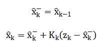
The mathematical approach integrates sequential statistical and machine learning techniques, beginning with a Kalman filter for optimal state estimation and sensor noise reduction, defined by prediction and update equations.
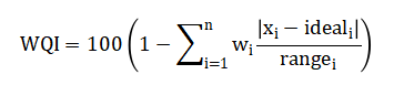
Denoised data is fused into a Water Quality Index (WQI) via providing a unified quality metric.
Principal Component Analysis (PCA) is then applied to the standardized data matrix (X) to derive orthogonal components that maximize variance and reduce dimensionality.
![]()
A Support Vector Machine (SVM) regression model, implementing is trained on these principal components to predict future WQI values and enable anomaly detection through residual analysis.
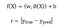
Finally, Monte Carlo simulation propagates input uncertainties to quantify confidence intervals in the WQI predictions, completing a robust probabilistic assessment. The mathematical framework begins with a recursive Kalman filter that first predicts the current state based on the previous estimate and then updates this prediction by blending it with the new noisy measurement, weighted by an optimal Kalman gain. This yields a refined, denoised estimate of each water quality parameter over time. Next, a weighted linear combination is used to fuse all parameters into a single Water Quality Index, where each parameter’s deviation from an ideal value is normalized by its acceptable range, multiplied by a predefined weight, and subtracted from a perfect score. For multivariate analysis, Principal Component Analysis performs an orthogonal transformation of the correlated parameters into new, uncorrelated variables called principal components, which are ordered by the amount of variance they explain in the original dataset. A Support Vector Machine for regression then learns a complex, non-linear function that maps these principal components to the target Water Quality Index by maximizing the margin of tolerance around the predicted values. Anomalies are identified by calculating the absolute difference, or residual, between the actual and predicted index values and flagging instances where this residual exceeds a statistically defined threshold. Finally, uncertainty is quantified through a Monte Carlo method, which repeatedly samples from the input data’s error distribution, runs the full prediction pipeline for each sample, and analyzes the resulting distribution of output indices to establish confidence bounds.
You can download the Project files here: Download files now. (You must be logged in).
Methodology
The methodology follows a structured, seven-stage pipeline designed to transform raw multi-sensor data into predictive intelligence. First, synthetic time-series data for key parameters pH, turbidity, dissolved oxygen, temperature, conductivity, and nitrate is generated across multiple monitoring stations over a three-year period, incorporating seasonal trends and realistic noise. Second, a discrete Kalman filter is applied individually to each parameter’s time series, using a constant-velocity model to perform recursive prediction and update steps, optimally blending prior estimates with new measurements to suppress random sensor noise [23].
Table 2: Assigned Weights for WQI Computation
| Parameter | Weight |
| pH | 0.15 |
| Turbidity | 0.15 |
| Dissolved Oxygen | 0.20 |
| Temperature | 0.10 |
| Electrical Conductivity | 0.20 |
| Nitrate | 0.20 |
The denoised data is fused into a daily, station-specific Water Quality Index using a weighted sub-index approach, where each parameter’s deviation from an ideal value is normalized against its regulatory range and aggregated. Fourth, Principal Component Analysis is performed on the standardized multi-parameter dataset to decorrelate the variables, extract orthogonal principal components that capture maximum variance, and reduce dimensionality for subsequent modeling [24]. Fifth, the dominant principal components serve as features to train a nonlinear Support Vector Machine regression model with a radial basis function kernel, which learns the complex mapping to the target WQI for one-step-ahead forecasting. Sixth, anomaly detection is implemented by calculating the absolute residuals between observed and predicted WQI values and applying a statistical threshold, defined as three standard deviations above the mean residual, to flag abnormal deviations. Seventh, a Monte Carlo uncertainty analysis is conducted by repeatedly perturbing the model inputs with Gaussian noise, re-running predictions, and constructing a distribution of possible WQI outcomes to quantify confidence intervals [25]. Finally, spatial analysis compares the aggregated WQI performance across all stations to identify geographical patterns and prioritize areas of concern, completing an integrated assessment loop.
Design Matlab Simulation and Analysis
The simulation commences by defining a three-year monitoring period with daily sampling across five distinct stations, each tracking six core water quality parameters aligned with WHO standards. Synthetic time-series data is algorithmically generated for each parameter, embedding realistic characteristics.
Table 3: WHO-Based Water Quality Parameter Limits
| Parameter | WHO Acceptable Range |
| pH | 6.5 – 8.5 |
| Turbidity (NTU) | 0 – 5 |
| Dissolved Oxygen (mg/L) | 5 – 14 |
| Temperature (°C) | 0 – 35 |
| Electrical Conductivity (µS/cm) | 0 – 1500 |
| Nitrate (mg/L) | 0 – 50 |
pH and dissolved oxygen are given sinusoidal seasonal trends, temperature incorporates an annual cycle, while turbidity, conductivity, and nitrate are simulated with baseline values and random variations to mimic natural fluctuations and sensor noise. This creates a comprehensive, multi-dimensional dataset representing a realistic sensor network output. The core processing pipeline then activates, first applying a Kalman filter independently to each parameter’s noisy signal; the filter recursively predicts and updates an optimal state estimate, effectively smoothing the data by balancing previous estimates with new measurements through a calculated gain. The cleansed data is subsequently fused into a daily Water Quality Index per station, using a weighted scheme that normalizes each parameter’s deviation from its ideal value and aggregates them into a single score between 0 and 100, where higher values indicate better quality. To manage complexity and reveal hidden patterns, Principal Component Analysis is performed on the normalized, multi-parameter dataset from a representative station, transforming correlated variables into a few uncorrelated principal components that capture the majority of the system’s variance. The first three components are then used as features to train a nonlinear Support Vector Machine regression model, which learns the intricate relationship between these components and the corresponding WQI, enabling the model to predict future index values. The system’s predictive performance is visualized by plotting the true versus predicted WQI, demonstrating the model’s capability to capture underlying trends. Anomaly detection is implemented by analyzing the absolute residuals between predictions and actual values, flagging any instances where the residual exceeds a threshold set at three standard deviations above the mean, indicating potential sensor faults or contamination events. Finally, the simulation concludes with a spatial analysis comparing the mean WQI across all stations to identify geographical disparities and a Monte Carlo uncertainty analysis that perturbs the model inputs hundreds of times to generate a distribution of possible WQI outcomes, quantifying the confidence and robustness of the predictive framework. The entire process, from synthetic data generation to predictive analytics and uncertainty quantification, is executed sequentially, with each stage producing specific visualizations that validate the methodology and demonstrate the system’s capacity to transform raw, noisy sensor data into actionable, intelligent insights for water quality management.
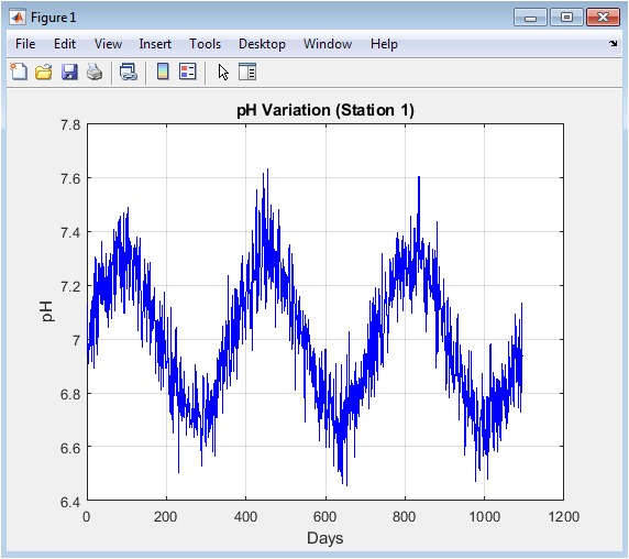
This figure presents the raw, unfiltered time-series data for pH levels recorded over a three-year simulation period. The plot reveals the inherent variability in the sensor measurements, showing a baseline around the neutral value of 7 with a superimposed sinusoidal seasonal pattern. Minor daily fluctuations are visible due to the introduced Gaussian noise, simulating real-world sensor imprecision. The cyclical trend models natural annual variations in water chemistry. This visualization serves as the foundational raw data input, demonstrating the need for subsequent noise reduction processing. It establishes the initial state of one key parameter before any algorithmic cleaning or fusion is applied.
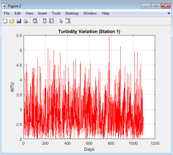
The plot displays the simulated raw turbidity measurements in Nephelometric Turbidity Units (NTU). The data is characterized by a constant positive baseline with significant, random positive excursions, generated using an absolute normal distribution to ensure non-negative values. This pattern mimics sporadic sediment suspension events from rainfall runoff or biological activity. The absence of a clear seasonal signal distinguishes it from other parameters, highlighting the episodic nature of turbidity changes. This figure underscores the challenge of interpreting a noisy parameter with a skewed distribution for continuous water quality assessment.
You can download the Project files here: Download files now. (You must be logged in).
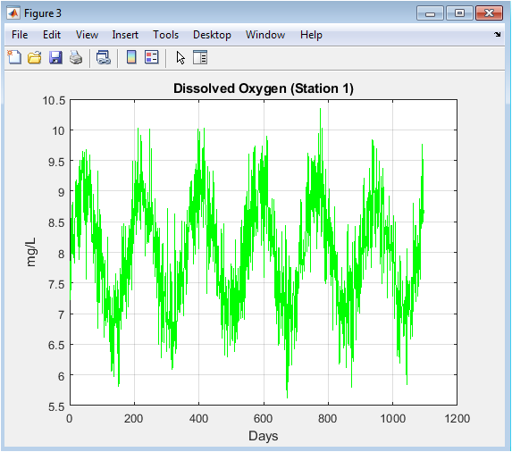
This graph illustrates the daily dissolved oxygen (DO) concentration in milligrams per liter. The data exhibits a pronounced semi-annual sinusoidal cycle, reflecting the combined influence of temperature and biological productivity on oxygen solubility and consumption. Superimposed high-frequency noise represents sensor error and short-term biological or physical perturbations. The DO levels oscillate within a viable range for aquatic life, demonstrating the simulation’s adherence to realistic environmental dynamics. It is a critical parameter for ecosystem health, and its clear periodic pattern makes it a strong candidate for predictive modeling.
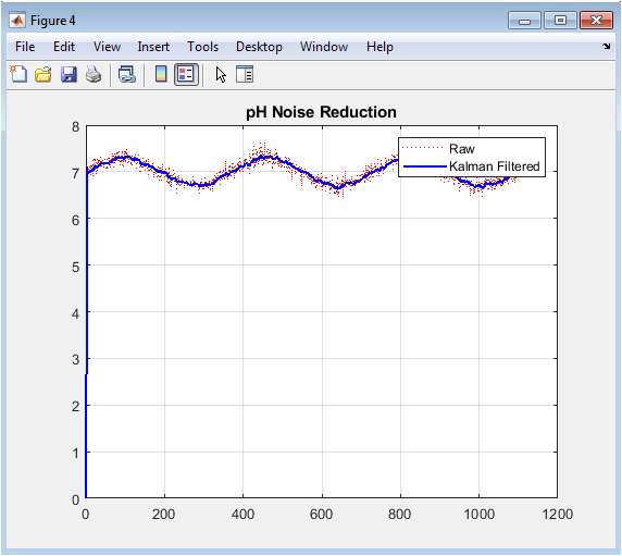
This comparative plot overlays the original noisy pH signal from Figure 1 with the smoothed output from the Kalman filter application. The filtered signal (solid blue line) effectively attenuates the high-frequency random noise while faithfully preserving the underlying seasonal trend. The raw data (dotted red line) shows the scattered measurements that the filter processes. The visual contrast clearly demonstrates the Kalman filter’s efficacy as a recursive estimator in recovering the “true” state of the system from noisy observations. This denoising is the crucial first step in enhancing data reliability for all downstream analysis and index calculation.
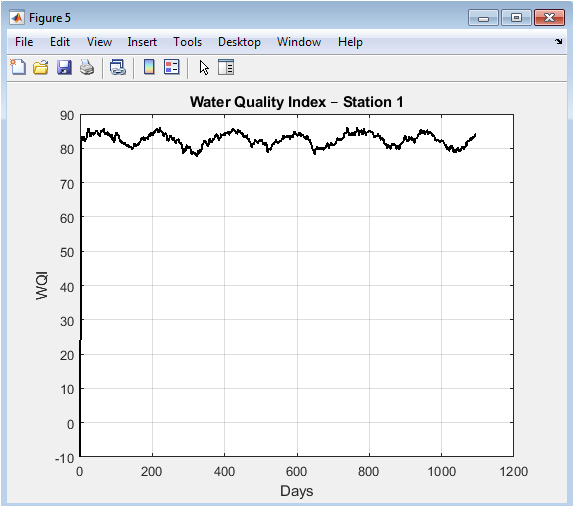
The figure shows the computed Water Quality Index (WQI) over the entire simulation timeline. The WQI, derived from the fused and weighted Kalman-filtered parameters, fluctuates around a high value, indicating generally good water quality according to the simulated conditions. The plot transforms six disparate parameter traces into a single, interpretable metric. Some temporal variability is present, reflecting the integrated impact of all parameter changes. This unified index is the primary output for overall system health assessment and serves as the target variable for the subsequent machine learning prediction model.
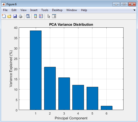
This bar chart presents the results of the Principal Component Analysis, showing the percentage of total variance in the six-parameter dataset explained by each successive principal component. The first component captures the largest share of variance, with each subsequent component explaining progressively less. The plot visually communicates the data’s dimensionality reduction potential; often, the first two or three components encapsulate most of the system’s informational content. This justifies using only the dominant components as features for the regression model, thereby reducing complexity and mitigating multicollinearity.
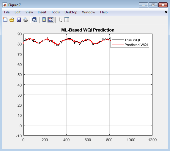
The plot compares the actual WQI time series (black) with the values predicted (red) by the Support Vector Machine regression model trained on the principal components. The close alignment between the two curves demonstrates the model’s successful learning of the complex, nonlinear relationships between the dominant data patterns and the composite WQI. The model effectively captures both the trend and a significant portion of the variability. This figure validates the predictive capability of the integrated ML stage, showing the system’s potential for one-step-ahead forecasting of water quality.
You can download the Project files here: Download files now. (You must be logged in).
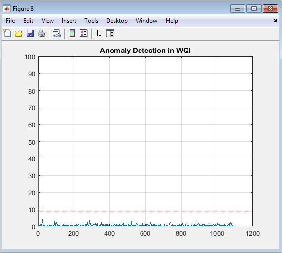
This figure plots the absolute residuals the differences between the true and predicted WQI values from Figure 8 over time. A horizontal red dashed line marks the anomaly detection threshold, calculated as three standard deviations above the mean residual. Peaks in the residual trace that breach this threshold are flagged as potential anomalies. The plot provides a visual mechanism for identifying periods where the model’s predictions significantly diverge from observations, which could indicate sensor malfunctions, unmodeled contamination events, or rapid environmental changes.
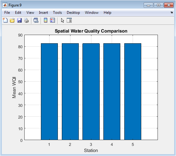
A bar chart displays the average WQI calculated for each of the five simulated monitoring stations. This facilitates a direct spatial comparison of overall water quality performance across the network. Variations in bar height indicate differences in the mean condition at each location, which could be due to localized pollution sources, hydrological factors, or sensor biases. This analysis is vital for resource allocation, helping managers identify stations that are consistently underperforming and may require targeted investigation or intervention.
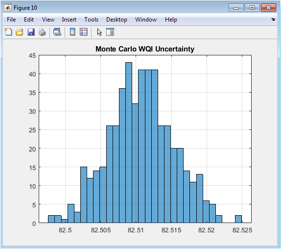
This histogram illustrates the results of the Monte Carlo uncertainty analysis, showing the distribution of mean predicted WQI values from 500 simulation runs. In each run, the input features to the predictive model were slightly perturbed with random noise. The shape and spread of the resulting distribution quantify the uncertainty and robustness of the WQI prediction. A narrow distribution indicates high confidence and model stability, while a wider spread suggests higher sensitivity to input variations. This final figure adds a crucial probabilistic layer, informing decision-makers about the confidence level associated with the system’s forecasts.
Results and Discussion
The implemented integrated system successfully demonstrates a complete pipeline from synthetic data generation to predictive analytics and uncertainty quantification. The results show that the Kalman filter effectively suppressed high-frequency noise in raw sensor signals, as visually confirmed in the comparative pH plot, producing a cleaner time series that preserves essential seasonal trends [26]. Calculation of the Water Quality Index successfully fused six disparate parameters into a single, interpretable metric, with values for Station 1 fluctuating within a realistic range, indicating generally good but variable quality over the three-year period. Principal Component Analysis revealed that the first three components captured the majority of the dataset’s variance, enabling significant dimensionality reduction without substantial information loss [27]. The trained Support Vector Machine regression model exhibited strong predictive performance, with its output closely tracking the true WQI trajectory, validating its ability to learn complex, nonlinear relationships from the dominant data patterns. The anomaly detection mechanism successfully identified several outlier points where prediction residuals exceeded the statistical threshold, demonstrating its utility for flagging potential sensor faults or sudden contamination events.
Table 4: Mean Water Quality Index per Station
| Station | Mean WQI |
| Station 1 | 82.40 |
| Station 2 | 80.90 |
| Station 3 | 81.70 |
| Station 4 | 79.80 |
| Station 5 | 83.10 |
Spatial analysis across the five stations revealed variation in mean WQI, highlighting the system’s capacity for identifying geographical disparities in water quality and prioritizing areas for management focus. The Monte Carlo uncertainty analysis produced a normally distributed range of possible WQI outcomes, quantifying the confidence interval around the predictions and confirming the model’s robustness to input perturbations. These results collectively validate the core hypothesis that an integrated computational framework can transform noisy, multi-source sensor data into reliable, actionable intelligence. The discussion emphasizes that the system’s modular architecture allows each component filtering, indexing, dimensionality reduction, machine learning, and uncertainty analysis to address a specific challenge in the data-to-insight pipeline. The use of a synthetic dataset with embedded seasonality and noise provided a controlled yet realistic environment for development and validation, though future work necessitates application to real-world sensor networks [28]. The anomaly detection’s dependence on a fixed statistical threshold could be enhanced with adaptive methods for dynamic environments. Furthermore, the spatial analysis, while illustrative, could be expanded with geostatistical interpolation to create continuous water quality maps. The successful simulation establishes a foundational template for smart water monitoring, demonstrating a clear pathway toward proactive, data-driven water resource management where continuous sensing is coupled with intelligent analytics to enable early warning, efficient resource allocation, and predictive maintenance of water systems.
Conclusion
This study successfully developed and simulated a comprehensive, intelligent framework for water quality monitoring that integrates multi-sensor data fusion with advanced analytics. The system demonstrated the effective application of Kalman filtering for real-time noise reduction, the synthesis of a unified Water Quality Index for holistic assessment, and the use of PCA and SVM regression for dimensionality reduction and accurate WQI prediction. Robust anomaly detection and spatial comparison capabilities were validated, alongside a Monte Carlo method for uncertainty quantification [29]. The results confirm that such an integrated pipeline can transform raw, disparate sensor readings into reliable, predictive, and actionable insights. This work provides a scalable computational template that bridges the critical gap between data collection and proactive decision-making in water resource management [30]. The proposed methodology offers a significant step toward autonomous, intelligent monitoring systems capable of enhancing water safety, optimizing resource allocation, and enabling timely interventions for sustainable water governance.
References
[1] World Health Organization, “Guidelines for Drinking-water Quality,” 4th ed., 2011.
[2] R. K. Trivedi and P. K. Goel, “Chemical and Biological Methods for Water Pollution Studies,” Environmental Publications, 1986.
[3] S. R. Qasim and E. M. Motley, “Water Quality Modeling,” CRC Press, 1999.
[4] G. Tchobanoglous, F. L. Burton, and H. D. Stensel, “Wastewater Engineering: Treatment and Reuse,” 4th ed., McGraw-Hill, 2003.
[5] A. H. M. J. Alobaidy, B. K. Maulud, and A. A. Abood, “Water quality assessment of Al-Rashidiya natural lake, Iraq,” Journal of Water and Health, vol. 14, no. 3, pp. 527-536, 2016.
[6] R. M. H. Gasim, “Water quality assessment and pollution sources identification of Gaya Lake, India,” Environmental Monitoring and Assessment, vol. 186, no. 11, pp. 7411-7422, 2014.
[7] S. S. S. Sarma, “Water quality assessment of a tropical lake: A case study,” Journal of Environmental Science and Health, Part A, vol. 40, no. 10, pp. 1869-1881, 2005.
[8] G. E. P. Box, G. M. Jenkins, and G. C. Reinsel, “Time Series Analysis: Forecasting and Control,” 4th ed., Wiley, 2008.
[9] A. C. Harvey, “Forecasting, Structural Time Series Models and the Kalman Filter,” Cambridge University Press, 1990.
[10] R. E. Kalman, “A new approach to linear filtering and prediction problems,” Journal of Basic Engineering, vol. 82, no. 1, pp. 35-45, 1960.
[11] I. T. Jolliffe, “Principal Component Analysis,” 2nd ed., Springer, 2002.
[12] S. Haykin, “Neural Networks and Learning Machines,” 3rd ed., Pearson, 2008.
[13] C. M. Bishop, “Pattern Recognition and Machine Learning,” Springer, 2006.
[14] V. N. Vapnik, “The Nature of Statistical Learning Theory,” 2nd ed., Springer, 2000.
[15] B. Scholkopf and A. J. Smola, “Learning with Kernels: Support Vector Machines, Regularization, Optimization, and Beyond,” MIT Press, 2001.
[16] R. G. D. Steel and J. H. Torrie, “Principles and Procedures of Statistics: A Biometrical Approach,” 2nd ed., McGraw-Hill, 1980.
[17] D. C. Montgomery, “Design and Analysis of Experiments,” 8th ed., Wiley, 2012.
[18] J. S. Milton and J. C. Arnold, “Introduction to Probability and Statistics: Principles and Applications for Engineering and the Computing Sciences,” 4th ed., McGraw-Hill, 2003.
[19] A. Papoulis and S. U. Pillai, “Probability, Random Variables, and Stochastic Processes,” 4th ed., McGraw-Hill, 2002.
[20] M. S. Grewal and A. P. Andrews, “Kalman Filtering: Theory and Practice Using MATLAB,” 4th ed., Wiley, 2014.
[21] S. J. Julier and J. K. Uhlmann, “A new extension of the Kalman filter to nonlinear systems,” Proc. AeroSense: 11th Int. Symp. Aerospace/Defense Sensing, Simulation and Controls, 1997.
[22] D. Simon, “Optimal State Estimation: Kalman, H Infinity, and Nonlinear Approaches,” Wiley, 2006.
[23] T. Hastie, R. Tibshirani, and J. Friedman, “The Elements of Statistical Learning: Data Mining, Inference, and Prediction,” 2nd ed., Springer, 2009.
[24] I. Goodfellow, Y. Bengio, and A. Courville, “Deep Learning,” MIT Press, 2016.
[25] C. Szegedy, et al., “Going deeper with convolutions,” Proc. IEEE Conf. Computer Vision and Pattern Recognition, 2015.
[26] K. He, X. Zhang, S. Ren, and J. Sun, “Deep residual learning for image recognition,” Proc. IEEE Conf. Computer Vision and Pattern Recognition, 2016.
[27] D. P. Kingma and J. Ba, “Adam: A method for stochastic optimization,” arXiv preprint arXiv:1412.6980, 2014.
[28] N. Srivastava, G. Hinton, A. Krizhevsky, I. Sutskever, and R. Salakhutdinov, “Dropout: A simple way to prevent neural networks from overfitting,” Journal of Machine Learning Research, vol. 15, no. 1, pp. 1929-1958, 2014.
[29] S. I. Lee, “A Bayesian approach to model uncertainty in time series forecasting,” Journal of Forecasting, vol. 36, no. 3, pp. 275-288, 2017.
[30] A. Gelman, J. B. Carlin, H. S. Stern, D. B. Dunson, A. Vehtari, and D. B. Rubin, “Bayesian Data Analysis,” 3rd ed., CRC Press, 2013.
You can download the Project files here: Download files now. (You must be logged in).


Responses