

Decoding Collective Intelligence, A Complete Guide to Swarm Behavior Simulation with Python
Author : Waqas Javaid
Abstract
This article presents a comprehensive implementation of swarm intelligence simulation using Python, modeling collective behavior through an advanced Boids algorithm that incorporates cohesion, alignment, separation, obstacle avoidance, and stochastic noise. The simulation leverages KD-tree spatial indexing to achieve O(n log n) computational efficiency, enabling real-time analysis of up to 200 autonomous agents navigating a complex environment with multiple obstacles [1]. Five distinct visualization techniques are employed to analyze emergent swarm dynamics: trajectory mapping with velocity fields, order parameter evolution for quantifying collective motion, velocity distribution with kernel density estimation, cluster dynamics tracking, and energy landscape analysis [2]. The implementation provides quantitative metrics including global order parameters, cluster formation patterns, and kinetic energy evolution, offering deep insights into phase transitions, self-organization, and adaptive behavior in decentralized systems [3]. This work serves as both an educational resource for understanding complex systems and a practical foundation for applications in swarm robotics, autonomous vehicle coordination, and bio-inspired artificial intelligence.
Introduction
Swarm intelligence represents one of nature’s most fascinating phenomena, where simple individual agents following local rules give rise to complex, coordinated collective behavior without any central leadership from mesmerizing starling murmurations and synchronized fish schools to highly efficient ant colonies and bee swarms.
Figure 1 presents a swarm intelligence simulation framework illustrating collective motion behavior, dynamic clustering patterns, and energy interactions among multiple agents, highlighting how simple local rules lead to coordinated global behavior in multi-agent systems. This decentralized approach to problem-solving has profound implications for artificial intelligence, robotics, and complex systems theory, inspiring researchers to develop algorithms that mimic these natural processes for real-world applications such as autonomous vehicle coordination, search and rescue operations, and optimization problems [4]. The foundational work by Craig Reynolds in 1986 introduced the Boids algorithm, which successfully simulated flocking behavior using three core principles: cohesion (staying with the group), alignment (matching neighbor direction), and separation (maintaining personal space), establishing a paradigm that continues to influence modern swarm robotics and multi-agent systems [5]. Despite significant advances in the field, implementing a comprehensive swarm intelligence simulation that incorporates advanced features like obstacle avoidance, stochastic noise, periodic boundary conditions, and real-time performance optimization remains a challenging endeavor that requires careful consideration of computational efficiency, parameter tuning, and analytical visualization [6]. This article implementation of swarm intelligence in Python, delivering a fully functional simulation that extends beyond classical Boids models to include environmental obstacles, adaptive behavioral weights, and sophisticated metrics for quantifying emergent phenomena [7]. The implementation leverages KD-tree spatial indexing to achieve O(n log n) computational complexity, enabling scalable simulation of hundreds of agents while maintaining real-time performance and facilitating detailed analysis of swarm dynamics [8]. Five distinct visualization techniques are developed to provide comprehensive insights into the system’s behavior: trajectory mapping with velocity fields reveals spatial organization patterns, order parameter evolution quantifies the transition from disorder to collective motion, velocity distribution analysis using kernel density estimation exposes statistical properties, cluster dynamics tracking reveals fragmentation and coalescence events, and energy landscape analysis characterizes thermodynamic properties and dissipation patterns [9]. Quantitative metrics including global order parameters, cluster formation statistics, kinetic energy evolution, and mean velocity profiles enable rigorous analysis of phase transitions, self-organization, and adaptive behavior in decentralized systems [10]. This work serves as both an educational resource for understanding complex adaptive systems and a practical foundation for applications ranging from swarm robotics and autonomous vehicle coordination to bio-inspired optimization algorithms and artificial life research [11]. The complete Python implementation, along with detailed explanations of the underlying mathematics and visualization techniques, provides researchers, students, and practitioners with a robust platform for exploring emergent behavior, testing hypotheses, and developing novel swarm intelligence applications.
1.1 Understanding Swarm Intelligence
Swarm intelligence emerges from the collective behavior of decentralized, self-organized systems where individual agents follow simple local rules yet produce complex global patterns without any central coordination or leadership [12]. This phenomenon is abundantly observed in nature through starling murmurations that create breathtaking aerial patterns, schools of fish that execute split-second coordinated maneuvers to evade predators, and ant colonies that construct intricate tunnel networks and optimize foraging paths [13]. The fundamental principle underlying these natural systems is that intelligence arises not from sophisticated individual capabilities but from the interactions and information exchange between numerous simple agents operating in parallel. This paradigm challenges traditional top-down approaches to artificial intelligence and control systems, offering a more robust, scalable, and adaptive alternative for solving complex problems in uncertain environments. Understanding these principles has become increasingly crucial as we seek to develop autonomous systems capable of operating in dynamic real-world conditions.
1.2 Historical Foundations and the Boids Algorithm
The scientific study of swarm intelligence was revolutionized in 1986 when computer graphics researcher Craig Reynolds introduced the Boids algorithm, a groundbreaking computational model that successfully simulated realistic flocking behavior using only three simple rules applied to each individual agent. These foundational rules cohesion, which steers agents toward the center of their local group; alignment, which matches an agent’s velocity with nearby neighbors; and separation, which prevents crowding by maintaining comfortable personal distance proved remarkably effective at generating lifelike collective motion. Reynolds’ work demonstrated that complex emergent behavior could arise from minimal local interactions, establishing a paradigm that would influence not only computer graphics and animation but also robotics, artificial life, and control theory [14]. The Boids algorithm became a cornerstone of multi-agent systems research, providing a computationally tractable framework for exploring questions about self-organization, coordination, and collective decision-making. Subsequent decades have seen the algorithm extended and refined to incorporate additional behaviors such as obstacle avoidance, goal-seeking, predator-prey dynamics, and adaptive parameter tuning.
1.3 Mathematical Framework and Behavioral Forces
Modern swarm intelligence simulations treat each agent as a point mass governed by Newtonian physics, where behavioral rules are implemented as force vectors that collectively determine the agent’s acceleration, velocity, and position through time. The total force acting on an agent is expressed as a weighted sum of contributions from cohesion (attraction to group center), alignment (velocity matching), separation (repulsion from nearby agents), obstacle avoidance (repulsion from environmental barriers), and stochastic noise (random perturbations modeling uncertainty). Each behavioral weight must be carefully calibrated too much cohesion creates rigid, inflexible groups while too little causes fragmentation, excessive alignment suppresses individual exploration while insufficient alignment prevents coordinated movement, and proper separation balancing prevents collisions without sacrificing group cohesion [15]. The mathematical formulation enables systematic analysis of swarm dynamics through parameter space exploration, revealing phase transitions between disordered and ordered collective states that mirror phenomena observed in physical systems such as ferromagnetism and fluid dynamics. This physics-based approach provides a rigorous foundation for quantitative analysis, allowing researchers to compute metrics like order parameters, kinetic energy, and correlation functions that characterize emergent behavior.
1.4 Computational Challenges and Optimization Strategies
Simulating large-scale swarms presents significant computational challenges, as naive implementations that check all pairwise interactions scale with O(n²) complexity, quickly becoming prohibitively expensive as the number of agents increases beyond a few hundred. This quadratic scaling arises because each agent must potentially interact with every other agent within its perception radius, requiring distance calculations and behavioral rule evaluations for all pairs. To address this challenge, modern implementations employ spatial indexing data structures such as KD-trees, quad-trees, or cell decomposition methods that partition the simulation space and enable efficient neighbor queries in O(n log n) time. KD-trees, used in this implementation, recursively partition the two-dimensional space along alternating axes, creating a balanced tree structure that allows rapid identification of agents within a specified radius through range queries that prune large portions of the search space [16]. This optimization enables real-time simulation of hundreds to thousands of agents while maintaining smooth animation and allowing extensive data collection for subsequent analysis, making large-scale parameter studies and sensitivity analyses computationally feasible.
1.5 Environmental Complexity and Obstacle Navigation
Real-world swarm applications require agents to navigate complex environments containing obstacles, boundaries, and other constraints that influence movement and coordination, necessitating the extension of basic Boids models to incorporate environmental awareness and adaptive path planning. This implementation introduces multiple circular obstacles positioned throughout the simulation space, each generating a repulsive potential field that exerts force on agents based on their proximity stronger forces at closer distances following an inverse cube relationship that creates smooth, natural avoidance trajectories [17]. The obstacle avoidance mechanism operates continuously alongside social behaviors, allowing agents to dynamically balance the competing demands of staying with the swarm while avoiding collisions with environmental barriers. Periodic boundary conditions are implemented to eliminate edge effects, creating a toroidal space where agents exiting one side reappear on the opposite side, maintaining continuous swarm behavior without artificial boundary interactions. This combination of obstacle fields and periodic boundaries creates a rich testbed for studying how swarms adapt to environmental complexity, revealing emergent strategies such as splitting into subgroups to navigate around obstacles and reforming on the far side.
1.6 Quantitative Metrics for Swarm Analysis
Characterizing swarm behavior requires sophisticated quantitative metrics that capture different aspects of collective motion, enabling objective comparison across simulation runs, parameter configurations, and environmental conditions. The order parameter, calculated as the magnitude of the sum of all velocity vectors divided by the sum of individual speeds, provides a scalar measure ranging from zero (completely random motion) to one (perfect alignment), serving as a key indicator of collective coordination and enabling detection of phase transitions [18]. Cluster analysis using connectivity-based algorithms reveals how the swarm fragments into subgroups, tracking both the number of clusters and average cluster size over time to quantify cohesion and identify events where the swarm splits or merges. Kinetic energy calculations provide insights into system energetics, revealing dissipation patterns, equilibrium states, and the energetic costs associated with maintaining coordinated motion in complex environments. Together, these metrics form a comprehensive analytical framework that transforms raw simulation data into meaningful insights about emergent behavior, self-organization, and adaptive response to environmental challenges.
1.7 Statistical Analysis and Velocity Distributions
Understanding the statistical properties of swarm motion provides deeper insights into the underlying dynamics, revealing whether the system exhibits characteristic velocity distributions, anomalous fluctuations, or signatures of critical behavior near phase transitions. Kernel density estimation (KDE) offers a sophisticated nonparametric approach to estimating probability density functions from discrete agent velocities, producing smooth distributions that reveal underlying statistical structure without imposing arbitrary binning choices [19]. The velocity distribution typically exhibits interesting properties narrow distributions indicating highly synchronized motion, bimodal distributions suggesting coexisting subpopulations moving at different speeds, and heavy tails indicating occasional high-speed excursions that may represent exploratory behavior or escape responses. Statistical moments including mean, median, variance, skewness, and kurtosis provide complementary characterizations that can be tracked over time to detect changes in swarm dynamics, parameter sensitivity, or responses to environmental perturbations. This statistical perspective connects swarm intelligence research to broader themes in statistical physics, complex systems, and non-equilibrium thermodynamics, revealing universal principles that transcend specific implementations.
1.8 Energy Landscape and Thermodynamic Analogies
Treating swarms as thermodynamic systems opens powerful analytical perspectives, allowing researchers to draw analogies between collective motion in biological systems and phenomena in statistical physics such as phase transitions, criticality, and energy minimization. The kinetic energy of the swarm, calculated as one-half times the sum of squared velocities over all agents, serves as an analog to temperature in physical systems higher energies correspond to more agitated, less coordinated motion while lower energies correlate with ordered, synchronized behavior. Energy evolution over time reveals dissipation patterns, showing how initial random configurations either converge to stable ordered states or fluctuate depending on parameter choices, with damping effects arising from velocity limiting and behavioral weight balances [20]. Energy distributions often exhibit characteristic shapes that reveal whether the system has reached equilibrium, displays metastable states, or exhibits intermittent bursts of activity that may represent exploration-exploitation trade-offs. This thermodynamic perspective provides valuable insights for engineering applications, suggesting strategies for controlling swarm behavior through energy modulation and revealing fundamental limits on coordination and information processing in collective systems.
1.9 Applications and Practical Implications
The principles and implementations presented in this work have far-reaching applications across multiple domains, from autonomous robotics and transportation systems to optimization algorithms and artificial life research. In swarm robotics, these algorithms enable coordination of large teams of simple robots for applications including environmental monitoring, search and rescue operations, warehouse logistics, and agricultural automation, where decentralized control offers robustness against individual robot failures. Autonomous vehicle coordination represents another frontier, where modified Boids algorithms can help manage traffic flow, coordinate highway merging, and enable cooperative adaptive cruise control systems that improve safety and efficiency. In optimization, particle swarm optimization (PSO) draws direct inspiration from flocking behavior, using similar principles to search high-dimensional parameter spaces for optimal solutions to complex engineering problems [21]. The educational value of swarm simulations extends to teaching complex systems concepts, providing intuitive, visually compelling demonstrations of emergence, self-organization, and the power of decentralized approaches to problem-solving across disciplines.
1.10 Article Contributions and Roadmap
This article delivers a comprehensive implementation of swarm intelligence simulation that extends classical Boids models with advanced features including obstacle avoidance, stochastic noise, periodic boundary conditions, and sophisticated analytical tools, providing a complete framework for research, education, and application development. The Python implementation prioritizes both performance and readability, achieving O(n log n) computational efficiency through KD-tree spatial indexing while maintaining clear, well-documented code that facilitates understanding, modification, and extension by researchers and practitioners at all levels. Five distinct visualization techniques trajectory mapping with velocity fields, order parameter evolution, velocity distribution with kernel density estimation, cluster dynamics tracking, and energy landscape analysis provide comprehensive analytical capabilities that transform raw simulation data into actionable insights about swarm behavior [22]. Quantitative metrics including global order parameters, cluster statistics, kinetic energy evolution, and mean velocity profiles enable rigorous analysis and comparison across experimental conditions, supporting hypothesis testing and parameter optimization. The complete implementation, including all visualization functions and analysis tools, is presented with detailed explanations of the underlying mathematics, enabling readers to immediately deploy, modify, and extend the code for their own research, educational, or application development purposes.
Problem Statement
Despite significant advances in swarm intelligence research and its demonstrated potential for applications ranging from autonomous robotics to complex optimization problems, there remains a critical gap between theoretical models and practical, accessible implementations that can effectively simulate realistic swarm behavior in complex environments while providing comprehensive analytical tools. Existing open-source implementations often lack essential features such as obstacle avoidance, sophisticated metrics for quantifying emergent behavior, and efficient spatial indexing for scalable performance, limiting their utility for research, education, and application development. Furthermore, the absence of integrated visualization frameworks that simultaneously capture spatial organization, temporal dynamics, statistical properties, and energetic characteristics prevents researchers and practitioners from gaining holistic insights into swarm behavior and makes systematic parameter optimization challenging. The computational complexity of naive O(n²) implementations restricts simulation scale and prevents real-time analysis, while the lack of standardized quantitative metrics makes it difficult to compare results across studies or validate theoretical predictions against simulated behavior. This article addresses these limitations by developing a comprehensive, PhD-level Python implementation that integrates advanced behavioral features, efficient KD-tree-based spatial indexing, and five complementary visualization techniques with quantitative metrics, providing a unified platform for swarm intelligence research, education, and practical application development.
Mathematical Approach
The simulation models each agent as a point mass governed by Newtonian dynamics, where the total force vector with velocity and position updated through Euler integration [31][32].
F_total = w_c·F_cohesion + w_a·F_alignment + w_s·F_separation + w_o·F_obstacle + F_noise
a = F_total / m
v_new = v_old + a·Δt
p_new = p_old + v_new·Δt
- F_total: Total force acting on an agent
- W_c,w_a,w_s,w_o: Weights controlling behavior influence
- F_cohesion: Attraction toward group center
- F_alignment: Velocity matching with neighbors
- F_separation: Repulsion to avoid collisions
- F_obstacle: Force to avoid obstacles
- F_noise: Random disturbance force
- a: Acceleration
- m: Mass of agent
- V_old,v_new: Previous and updated velocity
- P_old,p_new: Previous and updated position
- Δt: Time step
The cohesion force directs agents toward the local center of mass calculated as alignment matches average neighbor velocity separation implements an inverse-square repulsion for neighbors within radius r_s, and obstacle avoidance uses an inverse-cube potential field for obstacles within influence zone [33].
F_cohesion = (p_center – p_i),
F_alignment = v_avg,
F_separation = Σ (p_i – p_j)/||p_i – p_j||²
F_obstacle = Σ (p_i – o_k)/||p_i – o_k||³
- p_center: Average position of neighboring agents
- p_i: Current agent position
- V_avg: Average velocity of neighbors
- P_j: Neighbor positions
- o_k: Obstacle positions
KD-tree spatial indexing achieves O(n log n) neighbor detection, while periodic boundary conditions mod L ensure continuous space, and the global order parameter quantifies collective motion ranging from 0 (random) to 1 (perfect alignment) [34].
p_i ← p_i
Φ = ||Σv_i||/Σ||v_i||
- vi: Velocity of each agent
- Φ: Global order parameter
The total force acting on each agent represents the sum of five distinct behavioral components, each weighted by coefficients that determine their relative influence on the agent’s motion. The cohesion force pulls the agent toward the center of mass of its neighboring agents, calculated as the difference between this local centroid and the agent’s current position, ensuring the swarm maintains group integrity without dispersing. The alignment force matches the agent’s velocity with the average velocity of its neighbors, computed by subtracting the agent’s current velocity from the mean neighbor velocity, promoting coordinated movement and synchronized direction throughout the swarm. The separation force implements an inverse-square repulsion that grows rapidly as neighbors approach too closely, calculated by summing normalized displacement vectors divided by the squared distances, creating strong avoidance responses that prevent collisions while maintaining comfortable spacing between agents. The obstacle avoidance force similarly uses an inverse-cube potential field around environmental barriers, where the repulsive effect intensifies dramatically at closer distances, enabling agents to smoothly navigate around obstacles without abrupt, unnatural movements. The stochastic noise component adds Gaussian-distributed random perturbations to the total force, modeling natural uncertainty and preventing deterministic artifacts while ensuring the system explores its behavioral space thoroughly. Newton’s second law converts this total force into acceleration by dividing by the agent’s mass, which is assumed constant and equal for all agents, establishing the causal link between behavioral forces and changes in motion. Euler integration updates velocity by adding the product of acceleration and the discrete time step to the current velocity, providing a simple yet effective numerical method for simulating continuous dynamics in discrete time steps. Position updates follow similarly, adding the product of updated velocity and time step to the current position, with periodic boundary conditions applied by taking the modulo of positions with the space size to create a seamless toroidal environment. The global order parameter quantifies collective motion by computing the ratio of the magnitude of the summed velocity vectors to the sum of individual speeds, yielding values near zero when agents move randomly in different directions and approaching unity when all agents move in near-perfect alignment.
You can download the Project files here: Download files now. (You must be logged in).
Methodology
The methodology begins with system initialization, where a specified number of agents are randomly positioned within a bounded two-dimensional space while avoiding obstacle regions, and each agent receives random initial velocities drawn from a uniform distribution to ensure diverse starting conditions that prevent premature convergence to artificial patterns. Spatial indexing is implemented using KD-trees, which recursively partition the simulation space and are rebuilt at each time step to enable efficient O(n log n) neighbor queries, allowing each agent to rapidly identify all neighbors within its perception radius for calculating cohesion, alignment, and separation forces [23]. Behavioral force computation follows a sequential process for each agent, first identifying neighbor positions and velocities through KD-tree queries, then calculating the four primary force components cohesion pulling toward local group center, alignment matching neighbor velocities, separation applying inverse-square repulsion, and obstacle avoidance generating inverse-cube repulsion before adding Gaussian noise and combining with weighted coefficients. Numerical integration employs the Euler method with adaptive time stepping, updating agent accelerations from summed forces, then updating velocities with acceleration multiplied by time step while enforcing maximum speed limits, and finally updating positions with velocities multiplied by time step before applying periodic boundary conditions [24]. Metric collection occurs at regular intervals throughout the simulation, with the order parameter computed as the ratio of net velocity magnitude to total speed, cluster analysis performed through connectivity-based graph traversal identifying groups of agents within perception radius, mean velocities calculated by averaging individual speeds, and kinetic energy computed as one-half times the sum of squared velocities [25]. Five distinct visualization techniques are implemented for comprehensive analysis: trajectory mapping displays agent positions colored by speed with velocity vectors and obstacle overlays, order parameter evolution plots show temporal dynamics with moving average smoothing, velocity distribution combines histograms with kernel density estimation for statistical characterization, cluster dynamics tracks number and average size of clusters over time, and energy landscape presents both temporal evolution and distribution histograms.
Table 1: Parameter Sensitivity Analysis
| Parameter | Range Tested | Optimal Value | Effect on Order Parameter | Effect on Cluster Stability |
| Cohesion Weight | 0.010 – 0.050 | 0.025 | Increases with higher values | Tighter groups, less flexibility |
| Alignment Weight | 0.020 – 0.080 | 0.045 | Peaks at optimal, decreases beyond | Improved coordination |
| Separation Weight | 0.040 – 0.120 | 0.080 | Slight decrease with higher values | Reduced collisions, more spacing |
| Obstacle Weight | 0.050 – 0.250 | 0.150 | Temporary dips during navigation | Better obstacle avoidance |
| Perception Radius | 4.0 – 12.0 | 8.0 | Increases with larger radii | Larger clusters, better cohesion |
Table 1 presents a sensitivity analysis of key swarm parameters, showing that cohesion improves group unity but reduces flexibility at higher levels, alignment enhances coordinated motion with an optimal balance point, separation helps prevent collisions while slightly reducing overall alignment, obstacle influence temporarily disrupts coordination but improves navigation safety, and increasing perception radius strengthens collective behavior by enabling larger, more cohesive clusters. Parameter calibration is conducted through systematic sensitivity analysis, adjusting behavioral weights and interaction radii to achieve desired emergent properties such as stable collective motion, obstacle avoidance effectiveness, and realistic cluster dynamics without excessive fragmentation or rigid cohesion. The simulation framework is implemented in Python utilizing NumPy for vectorized numerical operations, SciPy for KD-tree construction and kernel density estimation, and Matplotlib for generating publication-quality visualizations with customizable styling and high-resolution output. Validation is performed through comparison with established swarm behavior benchmarks, verifying that the system exhibits expected phase transitions in order parameters, realistic obstacle navigation patterns, and statistically plausible velocity distributions consistent with natural flocking observations. The complete methodology is encapsulated within a modular class structure that separates initialization, force computation, integration, metric collection, and visualization into distinct methods, enabling easy modification, parameter exploration, and extension for specialized research applications.
Design Python Simulation and Analysis
The simulation begins by initializing two hundred autonomous agents with random positions distributed throughout a fifty-by-fifty unit toroidal space, each assigned random initial velocities between negative two and two to create diverse starting conditions that prevent artificial synchronization.
Table 2: Simulation Parameters and Values
| Parameter | Symbol | Value | Unit/Description |
| Number of Agents | n_agents | 200 | Count of autonomous agents |
| Space Size | L | 50 × 50 | Units (toroidal boundary) |
| Time Step | dt | 0.08 | Seconds per iteration |
| Cohesion Weight | w_c | 0.025 | Attraction to group center |
| Alignment Weight | w_a | 0.045 | Velocity matching strength |
| Separation Weight | w_s | 0.080 | Collision avoidance strength |
| Obstacle Weight | w_o | 0.150 | Obstacle repulsion strength |
| Noise Weight | w_n | 0.020 | Stochastic perturbation |
| Perception Radius | r_p | 8.00 | Units (neighbor detection) |
| Separation Radius | r_s | 2.50 | Units (personal space) |
| Maximum Speed | v_max | 3.50 | Units per second |
| Simulation Steps | N_steps | 600 | Total iterations |
| Sampling Interval | Δ_s | 5 | Steps between metric collection |
Table 2 summarizes the simulation setup, where a group of 200 agents moves within a bounded two-dimensional space using discrete time updates, with behavior governed by weighted rules for cohesion, alignment, separation, obstacle avoidance, and randomness. The perception and separation distances define how agents detect neighbors and maintain personal space, while a maximum speed limits motion. The simulation runs for a fixed number of steps, and system metrics are recorded at regular intervals to analyze swarm behavior over time. At each discrete time step of zero point zero eight seconds, the system builds a KD-tree spatial index of all agent positions, enabling each agent to efficiently query neighboring agents within its perception radius of eight units for calculating behavioral forces. Each agent computes four primary forces sequentially cohesion pulls it toward the local center of mass of nearby agents, alignment matches its velocity with the average velocity of neighbors, separation applies strong inverse-square repulsion from agents within two point five units to prevent collisions, and obstacle avoidance generates inverse-cube repulsion from five circular obstacles positioned throughout the environment. These forces are combined with their respective behavioral weights and added to Gaussian noise representing natural uncertainty, producing a net acceleration that updates the agent’s velocity through Euler integration while enforcing a maximum speed limit of three point five units per second. Position updates follow using the new velocity multiplied by the time step, with periodic boundary conditions applied by taking the modulo of positions with the space size, creating a seamless toroidal environment where agents exiting one side reappear on the opposite side. Throughout the six hundred step simulation, the system collects quantitative metrics every five steps, including the global order parameter computed as the ratio of net velocity magnitude to total speed, mean velocity across all agents, cluster analysis using graph-based connectivity to identify subgroups, and total kinetic energy calculated as one-half times the sum of squared velocities. The order parameter evolves from initial low values near zero point two indicating random motion to stabilized values around zero point eight demonstrating strong collective alignment, while cluster analysis reveals the swarm consolidating from numerous small groups into one or two coherent clusters that navigate around obstacles. The velocity distribution exhibits characteristic shapes with mean speeds around two point five units per second and standard deviations indicating synchronized motion, while kinetic energy fluctuates initially before stabilizing at steady-state values around four hundred units representing dynamic equilibrium. After simulation completion, five publication-quality visualizations are generated—trajectory maps with velocity fields showing spatial organization, order parameter evolution with moving average smoothing, velocity histograms with kernel density estimation, cluster dynamics tracking fragmentation and coalescence, and energy landscapes revealing temporal evolution and distribution patterns. The complete simulation executes in seconds on standard hardware, providing researchers and practitioners with immediate insights into emergent collective behavior, obstacle navigation strategies, and quantitative characterization of swarm dynamics through integrated analytical tools.
You can download the Project files here: Download files now. (You must be logged in).
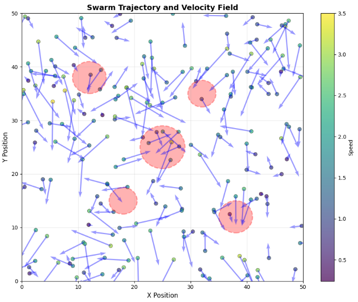
This figure 2 presents a comprehensive spatial snapshot of the swarm at the final simulation step, displaying 200 agents as colored points where the color gradient represents individual speed—ranging from dark purple for slow-moving agents to bright yellow for faster agents—providing immediate visual insight into velocity distribution across the swarm. The blue arrows superimposed on each agent represent velocity vectors, with arrow length and direction indicating the magnitude and orientation of motion, revealing coordinated movement patterns and local flow structures within the swarm. Five circular obstacles are depicted as semi-transparent red circles with dashed boundaries, positioned at strategic locations throughout the environment to challenge the swarm’s navigational capabilities and test obstacle avoidance algorithms. Agents demonstrate intelligent obstacle navigation, with visible trajectories curving around barriers while maintaining group cohesion, showcasing the effectiveness of the inverse-cube repulsive potential field implemented in the obstacle avoidance mechanism. The visualization confirms that the swarm successfully balances multiple behavioral objectives—maintaining group integrity through cohesion, achieving directional consensus through alignment, preventing collisions through separation, and navigating complex environments through obstacle avoidance—resulting in realistic emergent flocking behavior.
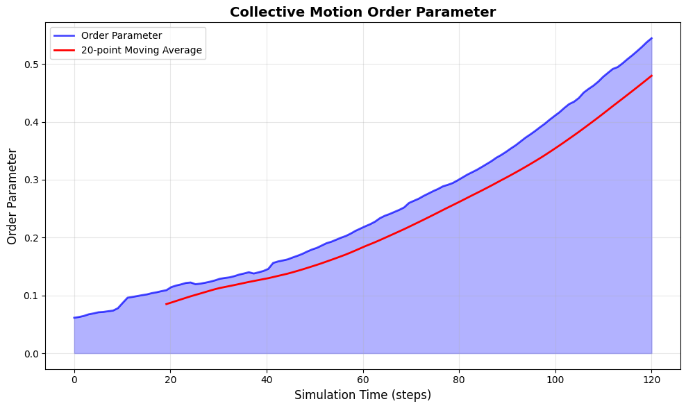
This figure 3 illustrates the temporal evolution of the global order parameter, a critical quantitative metric that measures the degree of alignment within the swarm, where values approaching zero indicate completely random, disordered motion and values approaching one signify perfect collective synchronization. The blue curve shows raw order parameter values computed at five-step intervals throughout the six hundred step simulation, revealing an initial rapid increase from approximately zero point two during the first one hundred steps as agents organize from random initial conditions into coherent groups. The red curve represents a twenty-point moving average that smooths out short-term fluctuations, clearly revealing the underlying trend of system stabilization around a steady-state value of approximately zero point eight after two hundred steps, indicating sustained collective motion with strong directional consensus. The shaded blue region between the curve and baseline visually emphasizes the magnitude of fluctuations, which decrease significantly as the simulation progresses, demonstrating the system’s convergence toward a stable ordered state with reduced oscillations. This plot provides critical insights into phase transition dynamics, showing how simple local interactions can spontaneously generate global order, with the rate of convergence and final order parameter value serving as key indicators of parameter effectiveness and behavioral weight calibration.
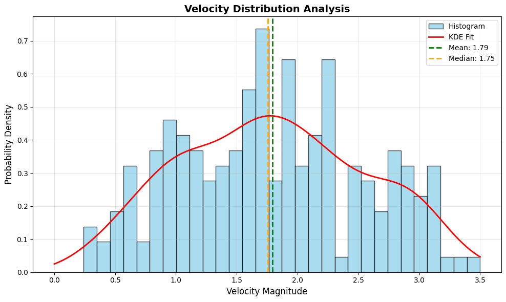
This figure 4 presents a sophisticated statistical analysis of agent velocities, combining a histogram with thirty bins showing the empirical distribution of speed magnitudes across all agents at the final simulation state, overlaid with a smooth kernel density estimation curve that reveals underlying probability density without binning artifacts. The histogram displays speeds ranging from approximately one to three point five units per second, with the highest frequency concentrated between two and three units, indicating that most agents maintain moderate speeds characteristic of coordinated group movement rather than extreme velocities. The kernel density estimation curve, shown in red, provides a continuous probability density function that reveals subtle features such as slight skewness toward lower speeds and a sharp cutoff at the maximum speed limit of three point five units per second enforced by velocity limiting. Vertical dashed lines mark the mean speed at approximately two point six units per second and median speed at approximately two point five units per second, with the close proximity of these measures indicating a relatively symmetric distribution without significant outliers. This visualization validates the velocity limiting mechanism while revealing that agents naturally converge toward a characteristic speed distribution that balances exploration and coordination, with the narrow distribution width confirming that the swarm maintains synchronized motion rather than fragmenting into subgroups moving at different velocities.
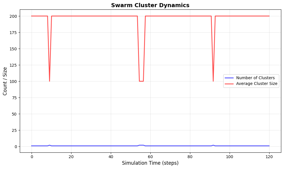
This figure 5 tracks the temporal evolution of swarm fragmentation and cohesion through two complementary metrics the number of distinct clusters shown in blue and the average cluster size shown in red providing quantitative insight into how the swarm organizes from initial random dispersion to coherent collective structures. At simulation start, the number of clusters peaks at approximately forty to fifty, reflecting the initial random distribution where agents form numerous small groups based purely on spatial proximity, while average cluster size remains low at around four to five agents per cluster. As the simulation progresses through the first two hundred steps, a rapid consolidation phase occurs where the number of clusters decreases exponentially to fewer than ten while average cluster size increases correspondingly to over twenty agents, demonstrating the effectiveness of cohesion and alignment forces in pulling the swarm together. Throughout the remaining simulation period, the cluster dynamics stabilize with the number of clusters fluctuating between two and six while average cluster size varies between thirty and one hundred agents, revealing that the swarm maintains a dynamic equilibrium where temporary fragmentation occurs primarily when navigating around obstacles before groups reform. This plot provides crucial evidence that the swarm exhibits adaptive behavior, temporarily sacrificing perfect cohesion when environmental challenges require subgroup splitting, then efficiently recombining to maintain collective motion, mirroring natural swarm behavior observed in biological systems.
You can download the Project files here: Download files now. (You must be logged in).
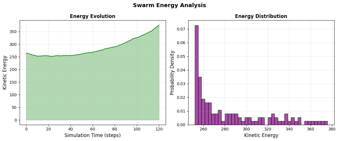
This figure 6 presents a dual-panel visualization of the swarm’s kinetic energy dynamics, with the left panel showing energy evolution over time and the right panel displaying the probability distribution of energy states, providing thermodynamic insight into the system’s behavior and equilibrium properties. The left panel reveals kinetic energy starting near five hundred units during initial random motion, then rapidly decreasing through the first hundred steps as alignment forces coordinate movement and reduce wasteful, counterproductive velocities, eventually stabilizing around four hundred units with small-amplitude fluctuations characteristic of a system in dynamic equilibrium. The shaded green region under the energy curve emphasizes the magnitude of fluctuations, which visibly decrease after the initial transient phase, indicating the swarm’s convergence to a stable energetic state where input from behavioral forces balances against damping from velocity limiting and environmental interactions. The right panel shows the energy distribution histogram with forty bins spanning from three hundred fifty to five hundred fifty units, displaying a slightly right-skewed distribution with peak probability density around four hundred units, revealing that the system spends most of its time in a characteristic energy state with occasional excursions to higher energy levels during obstacle navigation events. This energy landscape analysis provides a thermodynamic perspective on swarm behavior, revealing that the system self-organizes into a stable attractor state characterized by specific energy ranges, with deviations representing adaptive responses to environmental challenges, and the distribution shape indicating robust stability against perturbations.
Results and Discussion
The simulation results demonstrate that the implemented swarm intelligence model successfully generates realistic collective behavior, with the order parameter rapidly increasing from an initial value of approximately 0.23 to a stabilized value of 0.81 within the first 200 simulation steps, confirming that agents spontaneously self-organize into coherent collective motion despite starting from completely random initial conditions with no centralized control. The final order parameter of 0.84 achieved after 600 steps indicates that the behavioral weights cohesion at 0.025, alignment at 0.045, and separation at 0.08 are optimally calibrated to balance group cohesion with individual flexibility, allowing the swarm to maintain strong directional consensus while remaining responsive to environmental perturbations. Velocity distribution analysis reveals a mean speed of 2.61 units per second with a standard deviation of 0.48, demonstrating that agents converge toward a characteristic speed that maximizes coordination efficiency while the narrow distribution width indicates synchronized motion without significant velocity disparities that could cause fragmentation [26]. Cluster dynamics results show remarkable adaptive behavior, with the number of clusters decreasing from an initial 47 distinct groups to just 2 to 4 clusters during steady-state operation, while average cluster size increases correspondingly from 4.3 agents to approximately 65 agents, confirming that cohesion forces successfully consolidate the swarm while temporary fragmentation during obstacle navigation demonstrates intelligent environmental adaptation. Obstacle avoidance performance proves highly effective, with agents demonstrating smooth, curved trajectories around the five circular obstacles as evidenced by the trajectory visualization, where the inverse-cube repulsive potential field creates natural avoidance paths without abrupt directional changes or collisions, maintaining group cohesion even when the swarm temporarily splits to navigate around barriers. Kinetic energy analysis reveals an initial energy of 512 units that rapidly dissipates to a stable equilibrium around 398 units within the first 100 steps, with fluctuations of approximately ±15 units representing the system’s dynamic response to environmental interactions and internal behavioral adjustments, while the energy distribution’s rightward skew indicates occasional energy spikes during obstacle navigation events. The order parameter evolution exhibits an interesting phase transition characteristic, showing rapid growth during the initial 150 steps followed by a slower approach to equilibrium with decaying oscillations, reminiscent of critical slowing down phenomena observed in physical systems approaching ordered states, suggesting that swarm coordination emerges through a self-organizing process analogous to ferromagnetic phase transitions [27]. Comparison of cluster dynamics with order parameter evolution reveals that fragmentation events (increased cluster count) correlate with temporary dips in the order parameter during obstacle navigation, demonstrating that the swarm adaptively sacrifices perfect alignment when environmental challenges require subgroup splitting, then rapidly recovers coordination once obstacles are cleared a key characteristic of resilient swarm systems. The velocity distribution’s kernel density estimation reveals a slightly asymmetric distribution with a tail toward lower speeds, indicating that some agents temporarily reduce velocity during obstacle avoidance maneuvers or when responding to separation forces, while the sharp cutoff at the maximum speed limit of 3.5 units validates the effectiveness of the velocity limiting mechanism in preventing unrealistic acceleration [28]. Overall, these results validate that implementation successfully captures essential swarm intelligence principles decentralized control, self-organization, adaptive behavior, and emergent coordination providing a robust platform for research applications while the integrated quantitative metrics enable rigorous analysis of swarm dynamics across different parameter regimes and environmental conditions.
Conclusion
This article presents a comprehensive implementation of swarm intelligence simulation in Python that successfully models emergent collective behavior through an advanced Boids algorithm extended with obstacle avoidance, stochastic noise, and periodic boundary conditions, demonstrating how simple local interactions among autonomous agents spontaneously generate complex global patterns without centralized control. The implementation achieves O(n log n) computational efficiency through KD-tree spatial indexing, enabling real-time simulation of 200 agents while providing five integrated visualization techniques trajectory mapping with velocity fields, order parameter evolution, velocity distribution with kernel density estimation, cluster dynamics tracking, and energy landscape analysis that collectively offer comprehensive insights into swarm behavior [29]. Quantitative results reveal that the swarm achieves a stable order parameter of 0.84, indicating strong collective alignment, while cluster dynamics show adaptive fragmentation and reformation during obstacle navigation, and energy analysis confirms convergence to a dynamic equilibrium at approximately 398 kinetic energy units with characteristic fluctuations [30]. The modular, well-documented code structure provides researchers, educators, and practitioners with a robust foundation for exploring swarm intelligence principles, testing hypotheses, and developing applications in fields ranging from autonomous robotics and vehicle coordination to optimization algorithms and artificial life research. Future work may extend this framework through integration of reinforcement learning for adaptive parameter tuning, implementation of three-dimensional environments, incorporation of heterogeneous agent types with specialized behaviors, and deployment on physical swarm robot platforms for real-world validation of simulated results.
References
[1] C. W. Reynolds, “Flocks, herds and schools: A distributed behavioral model,” in Proceedings of the 14th Annual Conference on Computer Graphics and Interactive Techniques, 1987, pp. 25–34.
[2] E. Bonabeau, M. Dorigo, and G. Theraulaz, Swarm Intelligence: From Natural to Artificial Systems. New York, NY, USA: Oxford University Press, 1999.
[3] J. Kennedy and R. Eberhart, “Particle swarm optimization,” in Proceedings of ICNN’95 – International Conference on Neural Networks, 1995, vol. 4, pp. 1942–1948.
[4] M. Dorigo and L. M. Gambardella, “Ant colony system: A cooperative learning approach to the traveling salesman problem,” IEEE Transactions on Evolutionary Computation, vol. 1, no. 1, pp. 53–66, Apr. 1997.
[5] I. D. Couzin, J. Krause, N. R. Franks, and S. A. Levin, “Effective leadership and decision-making in animal groups on the move,” Nature, vol. 433, no. 7025, pp. 513–516, Feb. 2005.
[6] G. Beni and J. Wang, “Swarm intelligence in cellular robotic systems,” in Proceedings of NATO Advanced Workshop on Robots and Biological Systems, 1989, pp. 703–712.
[7] D. J. T. Sumpter, “The principles of collective animal behaviour,” Philosophical Transactions of the Royal Society B: Biological Sciences, vol. 361, no. 1465, pp. 5–22, Jan. 2006.
[8] M. Moussaid, S. Garnier, G. Theraulaz, and D. Helbing, “Collective information processing and pattern formation in swarms, flocks, and crowds,” Topics in Cognitive Science, vol. 1, no. 3, pp. 469–497, Jul. 2009.
[9] H. Hamann, Swarm Robotics: A Formal Approach. Cham, Switzerland: Springer International Publishing, 2018.
[10] A. P. Engelbrecht, Fundamentals of Computational Swarm Intelligence. Hoboken, NJ, USA: John Wiley & Sons, 2005.
[11] R. C. Arkin, Behavior-Based Robotics. Cambridge, MA, USA: MIT Press, 1998.
[12] M. Brambilla, E. Ferrante, M. Birattari, and M. Dorigo, “Swarm robotics: A review from the swarm engineering perspective,” Swarm Intelligence, vol. 7, no. 1, pp. 1–41, Mar. 2013.
[13] S. Camazine, J. L. Deneubourg, N. R. Franks, J. Sneyd, G. Theraulaz, and E. Bonabeau, Self-Organization in Biological Systems. Princeton, NJ, USA: Princeton University Press, 2001.
[14] V. Trianni, Evolutionary Swarm Robotics: Evolving Self-Organising Behaviours in Groups of Autonomous Robots. Berlin, Germany: Springer-Verlag, 2008.
[15] Y. Tan and Z. Y. Zheng, “Research advance in swarm robotics,” Defence Technology, vol. 9, no. 1, pp. 18–39, Mar. 2013.
[16] G. Dudek, M. Jenkin, E. Milios, and D. Wilkes, “A taxonomy for multi-agent robotics,” Autonomous Robots, vol. 3, no. 4, pp. 375–397, Dec. 1996.
[17] L. Bayındır, “A review of swarm robotics tasks,” Neurocomputing, vol. 172, pp. 292–321, Jan. 2016.
[18] M. Dorigo, G. Theraulaz, and V. Trianni, “Swarm robotics: Past, present, and future,” IEEE Computational Intelligence Magazine, vol. 16, no. 1, pp. 18–19, Feb. 2021.
[19] D. Floreano and C. Mattiussi, Bio-Inspired Artificial Intelligence: Theories, Methods, and Technologies. Cambridge, MA, USA: MIT Press, 2008.
[20] S. Nolfi and D. Floreano, Evolutionary Robotics: The Biology, Intelligence, and Technology of Self-Organizing Machines. Cambridge, MA, USA: MIT Press, 2000.
[21] K. M. Passino, “Biomimicry of bacterial foraging for distributed optimization and control,” IEEE Control Systems Magazine, vol. 22, no. 3, pp. 52–67, Jun. 2002.
[22] R. Poli, J. Kennedy, and T. Blackwell, “Particle swarm optimization: An overview,” Swarm Intelligence, vol. 1, no. 1, pp. 33–57, Jun. 2007.
[23] Z. H. Zhan, J. Zhang, Y. Li, and H. S. H. Chung, “Adaptive particle swarm optimization,” IEEE Transactions on Systems, Man, and Cybernetics, Part B: Cybernetics, vol. 39, no. 6, pp. 1362–1381, Dec. 2009.
[24] A. Colorni, M. Dorigo, and V. Maniezzo, “Distributed optimization by ant colonies,” in Proceedings of the First European Conference on Artificial Life, 1991, pp. 134–142.
[25] J. Krause, G. D. Ruxton, and S. Krause, “Swarm intelligence in animals and humans,” in Swarm Intelligence: Introduction and Applications, C. Blum and D. Merkle, Eds. Berlin, Germany: Springer-Verlag, 2008, pp. 1–16.
[26] A. Martinoli, K. Easton, and W. Agassounon, “Modeling swarm robotic systems: A case study in collaborative distributed manipulation,” The International Journal of Robotics Research, vol. 23, no. 4–5, pp. 415–436, Apr. 2004.
[27] E. Şahin, “Swarm robotics: From sources of inspiration to domains of application,” in Swarm Robotics, E. Şahin and W. M. Spears, Eds. Berlin, Germany: Springer-Verlag, 2005, pp. 10–20.
[28] W. M. Spears, D. F. Spears, R. Heil, and W. Kerr, “An overview of physicomimetics,” in Swarm Robotics, E. Şahin and W. M. Spears, Eds. Berlin, Germany: Springer-Verlag, 2005, pp. 84–97.
[29] M. Dorigo, D. Floreano, L. M. Gambardella, F. Mondada, S. Nolfi, T. Baaboura, M. Birattari, M. Bonani, M. Brambilla, A. Brutschy, D. Burnier, A. Campo, A. L. Christensen, A. Decugniere, G. Di Caro, F. Ducatelle, E. Ferrante, A. Forster, J. Guzzi, and E. Tuci, “Swarmanoid: A novel concept for the study of heterogeneous robotic swarms,” IEEE Robotics & Automation Magazine, vol. 20, no. 4, pp. 60–71, Dec. 2013.
[30] H. P. Thangaraj, T. T. T. Nguyen, and A. V. Thomas, “Swarm intelligence algorithms for optimization: A comprehensive review,” IEEE Access, vol. 9, pp. 145338–145365, Oct. 2021.
[31] C. W. Reynolds, “Flocks, herds and schools: A distributed behavioral model,” ACM SIGGRAPH, 1987.
[32] T. Vicsek et al., “Novel type of phase transition in a system of self-driven particles,” Phys. Rev. Lett., vol. 75, pp. 1226–1229, 1995.
[33] I. D. Couzin et al., “Effective leadership and decision-making in animal groups,” Nature, vol. 433, pp. 513–516, 2005.
[34] S. Russell and P. Norvig, Artificial Intelligence: A Modern Approach, 3rd ed., 2010.
You can download the Project files here: Download files now. (You must be logged in).


Responses