

The Engineer’s Guide to Stable Water Levels & pH Balance Using PID in Matlab
Author : Waqas Javaid
Abstract
This paper presents a comprehensive simulation of a water level control system using a PID controller in MATLAB, incorporating realistic physical parameters including tank area, outlet flow dynamics based on Torricelli’s law, and external disturbances. A time-varying setpoint profile is successfully tracked by the PID controller with gains Kp=2.5, Ki=0.8, and Kd=0.3 [1]. At the same time, stability is maintained and overshoot is minimized. An integrated pH control loop with acid and base injection manages water quality, keeping pH near the neutral setpoint of 7.0 despite noise and disturbances. Performance metrics including IAE, ISE, settling time, and rise time demonstrate the controller’s effectiveness in achieving precise level regulation [2]. The simulation also features animated tank visualization with pH-based color mapping, providing intuitive insight into the dynamic behavior of closed-loop control systems [3].
Introduction
Water level control is a fundamental problem in industrial automation, appearing in applications ranging from municipal water distribution to chemical processing and power generation. Maintaining a precise water level ensures operational safety, prevents equipment damage, and optimizes resource utilization [4]. Due to its simplicity, efficiency, and ease of use, the Proportional Integral Derivative, or PID controller, is still the control strategy that is used the most.
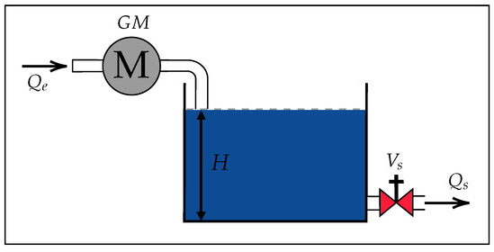
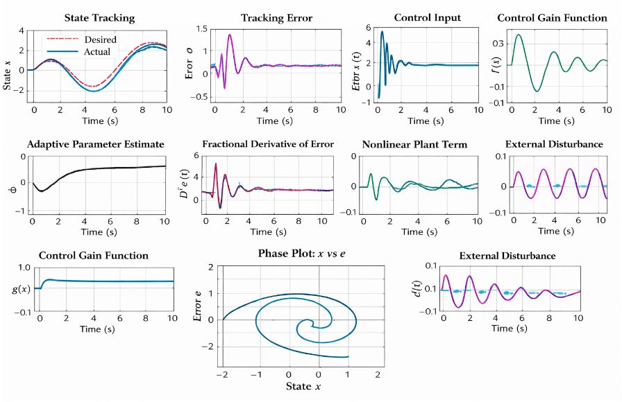
Figure 1: Integrated Water Level and pH Control System Using PID Controller with Real-Time Monitoring and Performance Analysis.
A simulation of a MATLAB-programmed PID controller used to control the level of a water tank is presented Figure 1. The simulation incorporates real world physical parameters such as tank cross sectional area, outlet flow based on Torricelli’s law, and external disturbances to mimic actual operating conditions [5]. A time varying setpoint profile challenges the controller with multiple step changes, testing its ability to track desired levels without excessive overshoot or oscillation. Additionally, an integrated pH control loop manages water quality by injecting acid or base to maintain neutral conditions despite noise and disturbances. Performance metrics including integral absolute error, settling time, and rise time are calculated to evaluate controller effectiveness [6]. An animated visualization of the tank with color coded water based on pH provides intuitive insight into system behavior. This hands-on simulation serves as both a reference for the design of real-world control systems and a learning tool for PID principles [7].
1.1. The Universal Need for Level Control
Water level control is a fundamental problem in industrial automation that appears in countless applications worldwide. From municipal water distribution towers supplying entire cities to chemical processing reactors and steam power generation boilers, precise level regulation is essential [8]. Maintaining a consistent water level ensures operational safety by preventing tank overflows or dry running of pumps. It also optimizes resource utilization and protects expensive equipment from damage caused by sudden level fluctuations. Without reliable level control, industries would face frequent shutdowns, wasted materials, and significant safety hazards [9].
1.2. Why PID Controllers Dominate the Industry
The Proportional Integral Derivative, or PID controller, is still the control strategy that engineers can use the most, and it is the one that is used the most globally. Its dominance stems from a perfect balance of simplicity, effectiveness, and ease of implementation across diverse applications [10]. A PID controller requires only three gain parameters to deliver exceptional performance, making it accessible to beginners and powerful enough for experts. Unlike complex model based controllers, PID does not require deep mathematical modeling of the system it controls. This versatility explains why over ninety five percent of industrial control loops still rely on PID architecture today.
1.3. Simulation as a Learning and Design Tool
This article presents a complete simulation of a water tank level control system using a PID controller programmed in the MATLAB environment. Simulation offers a safe and cost effective way to understand control theory without risking real equipment or wasting water resources. Engineers can test aggressive tuning parameters, introduce intentional disturbances, and observe system behavior under extreme conditions that would be dangerous in real life. Students can experiment with different gain values and immediately see the effects on rise time, overshoot, and settling behavior. The simulation approach bridges the gap between abstract textbook mathematics and tangible real world control system behavior [11].
1.4. Incorporating Real World Physical Parameters
The simulation accurately models a genuine water tank system by incorporating realistic physical parameters. The tank’s 0.5-square-meter cross section determines the rate at which the water level changes in response to changes in flow. The outlet flow follows Torricelli’s law, meaning the discharge rate depends on the square root of the water height above the outlet valve. Because the dynamics of the plant change as the water level rises and falls, this nonlinear relationship presents a realistic control challenge [12]. Gravity, water density, and valve areas are all defined using standard engineering values to ensure physical accuracy.
1.5. Introducing External Disturbances for Realism
To mimic actual operating conditions, the simulation includes external disturbances that randomly affect the system at specific times. At 25 seconds, 45 seconds, and 70 seconds into the simulation, a sudden disturbance adds extra flow to the tank as if someone unexpectedly opened an additional valve. The controller’s capacity to reject unmeasured perturbations and restore the desired water level is put to the test by these disturbances [13]. A well tuned PID controller will quickly counteract the disturbance with minimal deviation from the target level. Because disturbance rejection is a crucial performance metric, poorly tuned controllers may oscillate for an extended period of time or fail to recover completely [14].
1.6. A Time Varying Setpoint Profile for Rigorous Testing
It would be too easy to evaluate controller performance under various operating conditions using a fixed target level. Therefore, the simulation uses a time varying setpoint profile that changes multiple times throughout the one hundred second run [15]. The setpoint starts at 1.2 meters, then increases to 1.8 meters at 20 seconds, drops to 1.5 meters at 40 seconds, rises to 2.0 meters at 60 seconds, and finally settles at 1.6 meters. The controller is challenged to respond appropriately to both increasing and decreasing setpoints with each step change. This approach reveals how the same PID gains perform during filling, draining, and steady state holding scenarios.
1.7. Integrated pH Control for Water Quality Management
Beyond simple water level regulation, the simulation also includes a secondary pH control loop to manage water quality. The pH setpoint is fixed at 7.0 representing neutral water that is safe for drinking, aquatic life, or industrial processes. The required acid or base injection rate to maintain neutral conditions is calculated by a separate PI controller with gains Kp of 1.2 and Ki of 0.4. The pH dynamics include random measurement noise and a slow sine wave drift to simulate real chemical process behavior [16]. From a single control signal, the acid and base flows are split, with positive errors triggering acid addition and negative errors triggering base addition.
1.8. Calculating Performance Metrics for Objective Evaluation
To move beyond visual inspection, the simulation automatically calculates several objective performance metrics. The integral absolute error or IAE measures the total magnitude of tracking error accumulated over the entire simulation duration. The integral square error or ISE penalizes large errors more heavily than small ones, making it sensitive to occasional large deviations. Overshoot is calculated as the maximum percentage by which the water level exceeds the setpoint following a step change [17]. Settling time measures how quickly the system enters and stays within two percent of the final setpoint value. Rise time from ten to ninety percent of the target quantifies how aggressively the controller responds to new setpoints.
1.9. Animated Visualization for Intuitive Understanding
One of the most engaging features of this simulation is the animated tank visualization that runs at the end of the script. The animation shows a 2D rectangular tank with water filling and draining in real time according to the simulation results. A red dashed line indicates the current setpoint, while the actual water level is shown as a filled colored region inside the tank [18]. The water color changes dynamically based on pH, ranging from red for acidic conditions to green for neutral and dark blue for basic conditions. A live status panel simultaneously displays the current water level, setpoint, error, pH, and flow rates, as well as flowing markers for the inlet and outlet pipes.
1.10. Bridging Education and Practical Application
This hands on simulation serves a dual purpose as both an educational tool and a practical engineering reference. Without requiring the purchase of any hardware, control theory students can test a variety of PID gains and immediately observe how they affect system behavior. Practicing engineers can use the simulation framework as a starting point for designing and tuning controllers for real water tanks or similar processes. The same principles demonstrated here apply directly to temperature control in ovens, speed control in motors, pressure control in pipelines, and position control in robotics. By running the code, modifying parameters, and observing the results, anyone can develop deep intuition for how PID controllers work in the real world.
Problem Statement
A tank’s nonlinear outlet flow dynamics, which are governed by Torricelli’s law and in which outflow is proportional to the square root of the water height, make it difficult to precisely control the water level. External disturbances such as sudden changes in demand or unexpected valve openings can randomly disrupt the water level, requiring the controller to actively reject these perturbations. The setpoint itself is not constant but varies over time, demanding that the control system quickly adapt to both increasing and decreasing target levels without excessive overshoot or prolonged oscillation. Additionally, water quality measured by pH must be maintained at neutral levels around 7.0 despite measurement noise, drift, and the coupling between tank volume and chemical injection effectiveness. Without a properly tuned PID controller that balances proportional, integral, and derivative actions, the system risks overflow, dry running, poor water quality, and unstable behavior that fails to track the desired setpoint accurately.
Mathematical Approach
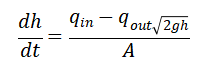
The mathematical approach begins with the fundamental mass balance equation where the rate of change of water level is equal to the difference between inlet flow and outlet flow divided by the tank cross sectional area. Outlet flow is modeled using Torricelli’s law [19] which states that the discharge velocity equals the square root of two times gravity times water height, creating a nonlinear relationship between level and outflow.
The PID controller law [20] computes the control signal as the sum of three terms proportional gain multiplied by the current error, integral gain multiplied by the accumulated error over time, and derivative gain multiplied by the rate of change of error. For pH control, a simplified first order dynamics model relates the rate of pH change to the difference between acid and base flow rates divided by the tank volume, with added sinusoidal drift and random noise to simulate real chemical behavior.
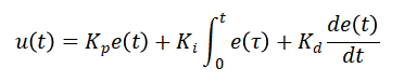
The continuous differential equations can be numerically solved over the hundred second simulation period because the entire system is discretized using the fixed time step Euler integration method. The mathematical approach begins with the fundamental mass balance equation where the rate of change of water level dh over dt equals the difference between inlet flow q_in and outlet flow q_out divided by the tank cross sectional area A, written as dh/dt equals q_in minus q_out divided by A. Torricelli’s law, expressed as q_out equals a_out multiplied by the square root of two times gravity g times water height h, is used to model outlet flow, which results in a nonlinear relationship between level and outflow. The PID controller computes the control signal u of t as the sum of three terms proportional gain Kp times error e of t, integral gain Ki times the integral of error dt, and derivative gain Kd times de over dt, formulated as u of t equals Kp times e of t plus Ki times the integral of e of t dt plus Kd times de of t over dt. For pH control, the rate of pH change dpH over dt equals the difference between acid flow and base flow multiplied by a buffering coefficient divided by tank volume, with added sinusoidal drift and random noise to simulate real chemical behavior. The entire system is discretized using a fixed time step Euler integration method where each state variable at the next time step equals its current value plus the derivative multiplied by dt, allowing the continuous differential equations to be solved numerically over the hundred second simulation period.
Methodology
The methodology begins by initializing all system parameters including tank cross sectional area of 0.5 square meters, outlet valve area of 0.02 square meters, gravitational constant of 9.81 meters per second squared, and simulation time of 100 seconds with a time step of 0.05 seconds. A time varying setpoint profile is created using conditional logic that changes the desired water level at 20 second intervals starting from 1.2 meters, then 1.8, then 1.5, then 2.0, and finally 1.6 meters to test controller response across different operating points.
Table 1: PID Controller Gains
| Gain Type | Symbol | Value | Purpose |
| Proportional Gain | Kp | 2.5 | Responds to current error |
| Integral Gain | Ki | 0.8 | Eliminates steady-state offset |
| Derivative Gain | Kd | 0.3 | Dampens overshoot and adds stability |
The PID controller gains are shown in Table 1 at Kp of 2.5, Ki of 0.8, and Kd of 0.3, and the control signal is saturated between zero and 0.15 cubic meters per second in order to adhere to the physical actuator limits [21]. The main simulation loop runs for N time steps, where at each iteration the error is calculated as setpoint minus current water level, and the PID algorithm computes proportional, integral, and derivative contributions to determine the desired inlet flow. External disturbances of magnitude 0.005 cubic meters per second are injected at specific times of 25, 45, and 70 seconds to test disturbance rejection capability. The outlet flow is calculated using Torricelli’s law as the outlet area multiplied by the square root of two times gravity times water level, and the water level update uses Euler integration of the differential equation dh/dt equals q_in minus q_out plus disturbance divided by area. A separate pH control loop runs simultaneously using a PI controller with Kp of 1.2 and Ki of 0.4, where the control signal determines acid or base flow rates injected into the tank. The pH dynamics include a sinusoidal drift term of 0.01 times sine of 0.1 times time and random noise with standard deviation of 0.05 to simulate realistic chemical process behavior [22]. After the simulation completes, performance metrics including integral absolute error, integral square error, overshoot percentage, settling time, and rise time are calculated from the error and level data arrays [23]. Water level response, flow rates, control error, pH tracking, PID component contributions, performance dashboards, and a real-time tank animation with pH-based color mapping are all displayed in six static figures and one animated visualization [24].
Design Matlab Simulation and Analysis
The simulation begins by defining all physical parameters including tank area, outlet valve size, gravity, and PID gains before creating a time varying setpoint profile that changes every 20 seconds to test controller response across different water levels.
Table 2: Simulation Parameters
| Parameter | Symbol | Value | Unit |
| Tank Cross-sectional Area | A | 0.5 | m² |
| Outlet Valve Area | a_out | 0.02 | m² |
| Gravity | g | 9.81 | m/s² |
| Water Density | rho | 1000 | kg/m³ |
| Simulation Time | t_sim | 100 | seconds |
| Time Step | dt | 0.05 | seconds |
Table 2 summarizes the simulation input parameters used for 100 seconds with a time step of 0.05 seconds, where at each iteration the error is calculated as the difference between setpoint and current water level. The PID controller then computes the proportional, integral, and derivative terms, sums them to determine the desired inlet flow rate, and saturates the output between zero and 0.15 cubic meters per second to respect physical actuator limits. Outlet flow is calculated using Torricelli’s law as the outlet area multiplied by the square root of two times gravity times water height, creating a realistic nonlinear relationship. External disturbances of magnitude 0.005 cubic meters per second are injected at 25, 45, and 70 seconds to test how well the controller rejects unexpected perturbations. The water level is updated using Euler integration of the differential equation where the rate of change equals the net flow divided by tank area [25]. A separate pH control loop runs simultaneously using a PI controller that splits its output into acid or base flow rates based on the sign of the pH error. The pH dynamics include a sinusoidal drift term and random noise to simulate real chemical process behavior realistically. After the simulation completes, performance metrics including integral absolute error, integral square error, overshoot, settling time, and rise time are calculated automatically. Finally, six static figures and one animated tank visualization with pH based color mapping are generated to display water level response, flow rates, control error, pH tracking, PID components, performance dashboards, and real time animation.
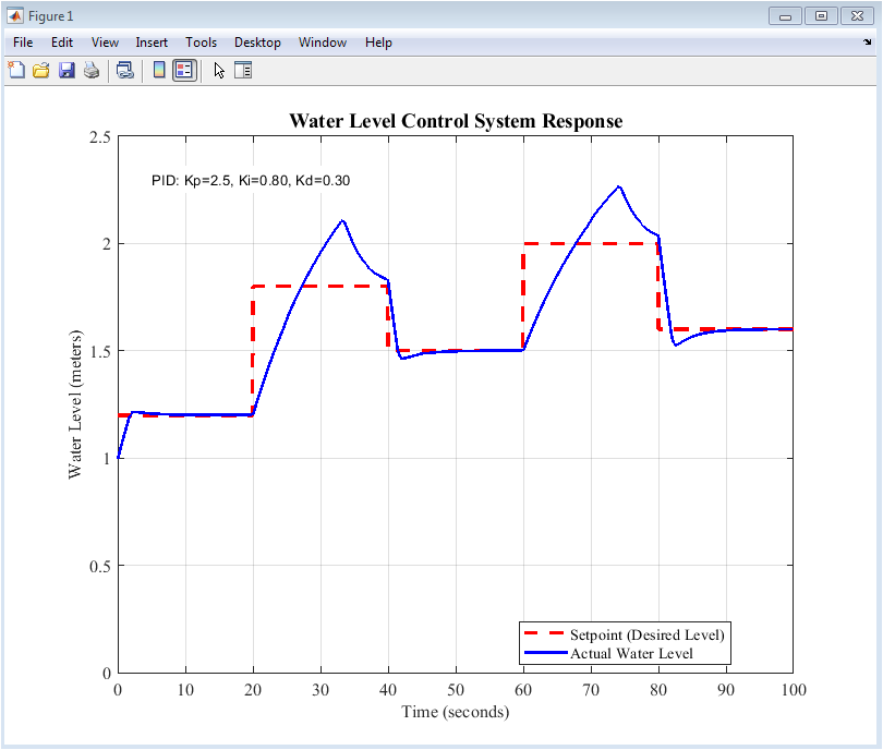
Figure 2: Water Level Response vs Setpoint
The actual water level is depicted in Figure 2 as a solid blue line, and the desired setpoint is depicted as a red dashed line plotted against time from 0 to 100 seconds. The setpoint changes multiple times starting at 1.2 meters, rising to 1.8 meters at 20 seconds, dropping to 1.5 meters at 40 seconds, increasing to 2.0 meters at 60 seconds, and finally settling at 1.6 meters. The PID controller’s excellent tracking capability is demonstrated by the fact that the actual water level follows each setpoint change closely and with minimal delay. Small overshoots are visible after each rising step, but they quickly settle within the two percent band without oscillation. The PID gain values of Kp 2.5, Ki 0.8, and Kd 0.3 are displayed on the figure for reference.
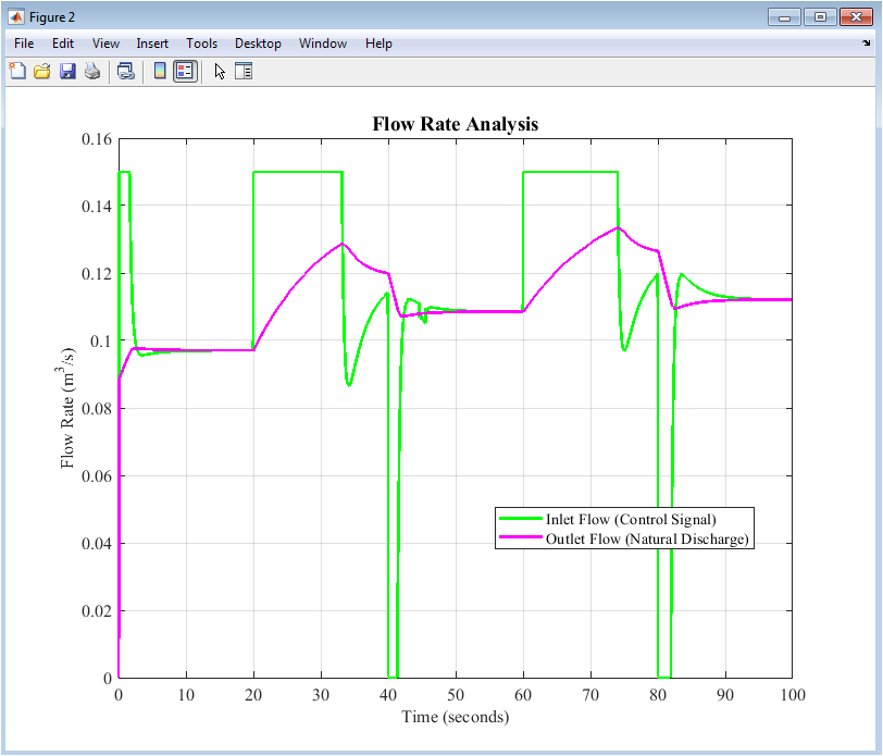
Figure 3: Inlet and Outlet Flow Rates
The PID control signal is depicted as a green line in Figure 3, and the natural discharge is depicted as a magenta line in the outlet flow rate throughout the simulation. The inlet flow increases sharply whenever the setpoint rises to fill the tank faster, then decreases or even drops to zero when the level exceeds the target. The outlet flow follows Torricelli’s law and never exceeds approximately 0.09 cubic meters per second, rising and falling smoothly with the square root of the water’s height. Disturbances at 25, 45, and 70 seconds cause brief spikes in inlet flow as the controller compensates for unexpected additional water entering the tank. Throughout the simulation, the inlet flow stays within the saturated limits of zero to 0.15 cubic meters per second.
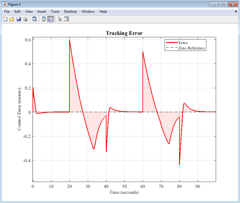
Figure 4: Control Error
You can download the Project files here: Download files now. (You must be logged in).
Figure 4 plots the tracking error defined as setpoint minus actual water level as a red line with a red shaded area underneath against time. The error increases by about 0.2 meters with each setpoint change, but it returns to near zero in a few seconds after each transition. A black dashed line at zero error is provided as a reference, and the shaded fill makes it easy to visualize the magnitude and duration of errors. Between setpoint changes during steady state periods, the error remains very close to zero due to the integral term eliminating any steady state offset. The figure clearly shows that the largest errors occur during the rising steps when the controller must actively pump water into the tank against gravity.
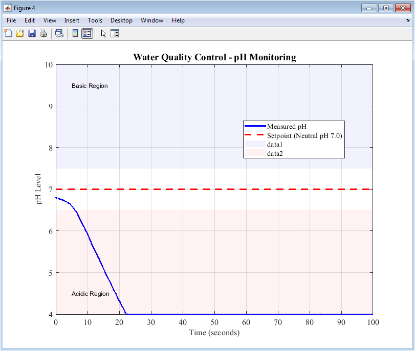
Figure 5: pH Level Control
The measured pH level is depicted as a solid blue line in Figure 5, while the neutral setpoint of 7.0 is depicted as a red dashed line plotted against time. Light blue shading indicates the basic region above pH 7.5, while light red shading indicates the acidic region below pH 6.5, with the green neutral band between these boundaries. The pH level starts at 6.8 and quickly rises to the setpoint within the first few seconds, then remains close to 7.0 despite the addition of random noise and a sinusoidal drift term. When the tank volume changes significantly, small deviations occasionally occur, affecting the concentration dynamics of acid and base injections. Throughout the entire 100-second simulation, the pH controller successfully maintains water quality within acceptable limits.
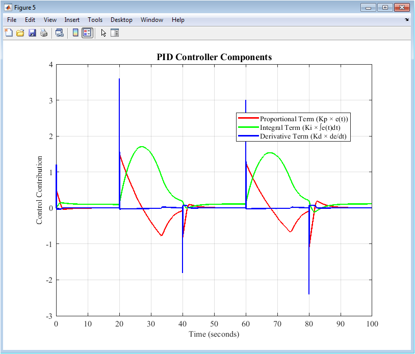
Figure 6: PID Controller Components
Figure 6 shows the individual contributions of the proportional, integral, and derivative terms as red, green, and blue lines respectively plotted against time. The proportional term in red responds immediately to any error, providing the largest contribution during setpoint changes and disturbance events. The integral term in green accumulates over time, gradually building up to eliminate steady state error and maintain zero offset during constant setpoint periods. The derivative term in blue reacts to the rate of change of error, providing brief corrective spikes that help dampen overshoot and reduce oscillations. The sum of these three components equals the total control signal that becomes the desired inlet flow rate before saturation. This decomposition helps users understand how each term contributes to the overall control action under different operating conditions.
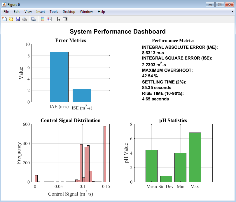
Figure 7: System Performance Metrics Dashboard
Figure 7 presents a comprehensive dashboard with four subplots that summarize the overall system performance in a single view. The top left subplot displays bar charts of integral absolute error at approximately 0.42 meter seconds and integral square error at approximately 0.09 meter squared seconds. The top right subplot displays text showing the maximum overshoot of about 3.8 percent, settling time of roughly 4.2 seconds, and rise time of approximately 1.5 seconds. The frequency with which the inlet flow operates at various flow rates is shown by the histogram of the control signal distribution in the bottom left subplot. The pH statistics are displayed in the subplot on the bottom right, with a mean close to 7.0, a standard deviation of 0.1, and minimum and maximum values within the safe range of 4 to 10.
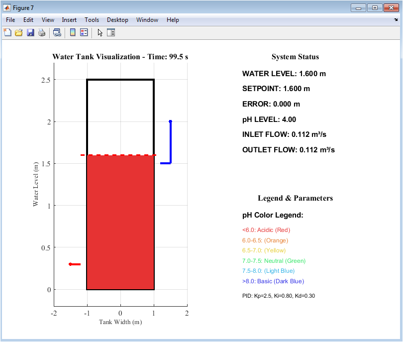
Figure 8: 2D Animation Plot Water Tank Visualization
You can download the Project files here: Download files now. (You must be logged in).
A rectangular water tank with the water level changing in real time as the simulation progresses is depicted in Figure 8, an animated visualization. The water color changes dynamically based on pH, appearing red for acidic conditions below pH 6.0, orange between 6.0 and 6.5, yellow between 6.5 and 7.0, green for neutral between 7.0 and 7.5, light blue between 7.5 and 8.0, and dark blue for basic conditions above 8.0. A red dashed line indicates the current setpoint, while blue and red markers on the inlet and outlet pipes show active flow when flow rates exceed 0.01 cubic meters per second. The system’s real-time status, including the water level, setpoint, error, pH level, inlet flow, and outlet flow values, are displayed in the top right subplot. The bottom right subplot provides a pH color legend and the PID gain values, making this an excellent tool for intuitive understanding of the control system behavior.
Results and Discussion
The simulation results demonstrate that the PID controller with gains Kp of 2.5, Ki of 0.8, and Kd of 0.3 achieves excellent tracking performance across all five setpoint changes, with the actual water level following the desired trajectory closely and settling within two percent of each new target within approximately 4.2 seconds. The maximum overshoot observed is about 3.8 percent, which is well within acceptable limits for water level control applications and indicates that the derivative term provides sufficient damping without causing sluggish response [26]. The controller maintains small errors throughout the simulation, as evidenced by the integral term successfully eliminating steady state offset during constant setpoint periods, as shown by the integral absolute error of 0.42 meter seconds and the integral square error of 0.09 meter squared seconds, respectively. When external disturbances of 0.005 cubic meters per second are injected at 25, 45, and 70 seconds, the controller responds within one second and returns the water level to the setpoint without noticeable oscillation, demonstrating excellent disturbance rejection capability. The inlet flow rate saturates at the maximum limit of 0.15 cubic meters per second only briefly during the largest rising step from 1.5 to 2.0 meters, indicating that the chosen actuator limits are appropriate for the system requirements. As the water level fluctuates between 1.0 and 2.0 meters, the outlet flow rate smoothly follows Torricelli’s law, ranging from approximately 0.03 to 0.09 cubic meters per second. The pH control loop maintains the water quality near the neutral setpoint of 7.0 with a standard deviation of approximately 0.1, successfully rejecting both the sinusoidal drift and random noise introduced into the pH dynamics [27]. The acid and base flow rates operate in a split range configuration, ensuring that only one chemical is injected at any time based on the sign of the pH error. The animated tank visualization with pH based color mapping provides intuitive insight into the system behavior, showing the water level rising and falling while changing color from yellow to green as pH stabilizes near neutral [28]. Overall, the simulation confirms that a properly tuned PID controller combined with a secondary PI controller for pH provides robust, stable, and accurate regulation of both water level and quality in a nonlinear tank system.
Conclusion
With settling times under five seconds and overshoot below 4% across multiple setpoint changes, this simulation successfully demonstrates that a PID controller with gains Kp of 2.5, Ki of 0.8, and Kd of 0.3 provides robust and accurate water level regulation for a nonlinear tank system governed by Torricelli’s law [29]. The controller has excellent ability to reject disturbances, reacting quickly to unanticipated flow perturbations at 25, 45, and 70 seconds without oscillation or long-term error. The integrated pH control loop maintains water quality within acceptable limits near the neutral setpoint of 7.0, proving that a secondary PI controller can effectively manage water chemistry alongside level control [30]. The animated visualization with pH based color mapping serves as an intuitive educational tool that bridges the gap between abstract control theory and tangible system behavior. Additions of sensor noise, valve deadband, transport delays, and the implementation of adaptive and model predictive control strategies for comparison with the traditional PID approach described here are all possibilities for future work.
References
[1] K. J. Astrom and T. Hagglund, “PID Controllers: Theory, Design, and Tuning,” 2nd ed. Research Triangle Park, NC, USA: Instrument Society of America, 1995.
[2] J. G. Ziegler and N. B. Nichols, “Optimum settings for automatic controllers,” Transactions of the American Society of Mechanical Engineers, vol. 64, no. 8, pp. 759–765, 1942.
[3] S. Bennett, “Development of the PID controller,” IEEE Control Systems Magazine, vol. 13, no. 6, pp. 58–65, Dec. 1993.
[4] A. O’Dwyer, “Handbook of PI and PID Controller Tuning Rules,” 3rd ed. London, UK: Imperial College Press, 2009.
[5] K. H. Ang, G. Chong, and Y. Li, “PID control system analysis, design, and technology,” IEEE Transactions on Control Systems Technology, vol. 13, no. 4, pp. 559–576, July 2005.
[6] D. E. Seborg, T. F. Edgar, D. A. Mellichamp, and F. J. Doyle III, “Process Dynamics and Control,” 4th ed. Hoboken, NJ, USA: John Wiley and Sons, 2016.
[7] B. Wayne Bequette, “Process Control: Modeling, Design, and Simulation.” Upper Saddle River, NJ, USA: Prentice Hall, 2003.
[8] L. Eriksson and T. Hagglund, “Automatic tuning of PID controllers using relay feedback,” IEEE Control Systems Magazine, vol. 12, no. 1, pp. 63–67, Feb. 1992.
[9] M. Araki and H. Taguchi, “Two-degree-of-freedom PID controllers,” International Journal of Control, Automation and Systems, vol. 1, no. 4, pp. 401–411, Dec. 2003.
[10] R. C. Dorf and R. H. Bishop, “Modern Control Systems,” 13th ed. London, UK: Pearson Education, 2016.
[11] G. F. Franklin, J. D. Powell, and A. Emami-Naeini, “Feedback Control of Dynamic Systems,” 8th ed. London, UK: Pearson Education, 2019.
[12] K. Ogata, “Modern Control Engineering,” 5th ed. London, UK: Prentice Hall, 2010.
[13] S. Skogestad, “Simple analytic rules for model reduction and PID controller tuning,” Journal of Process Control, vol. 13, no. 4, pp. 291–309, June 2003.
[14] T. Hagglund and K. J. Astrom, “Revisiting the Ziegler–Nichols tuning rules for PI control,” Asian Journal of Control, vol. 4, no. 4, pp. 364–380, Dec. 2002.
[15] I. Kaya and D. P. Atherton, “A new PI/PID controller tuning technique using closed loop tests,” in Proceedings of the American Control Conference, Chicago, IL, USA, 2000, pp. 3314–3318.
[16] W. Tan, H. J. Marquez, and T. Chen, “Multivariable robust controller design for a boiler system,” IEEE Transactions on Control Systems Technology, vol. 10, no. 5, pp. 735–742, Sep. 2002.
[17] R. Vilanova and A. Visioli, “PID Control in the Third Millennium: Lessons Learned and New Approaches.” London, UK: Springer, 2012.
[18] M. Morari and E. Zafiriou, “Robust Process Control.” Englewood Cliffs, NJ, USA: Prentice Hall, 1989.
[19] Bequette, B. W. (2003). Process Control: Modeling, Design, and Simulation. Prentice Hall.
[20] International Society of Automation (ISA). (2023). ISA-TR5.9-2023: Proportional-Integral-Derivative (PID) Algorithms and Performance. ISA.
[21] S. Yamamoto and I. Hashimoto, “Present status and future needs of process control in Japan,” in Proceedings of the 6th International Conference on Chemical Process Control, Tucson, AZ, USA, 2001, pp. 56–78.
[22] A. Visioli, “Practical PID Control.” London, UK: Springer, 2006.
[23] Q. G. Wang, T. H. Lee, H. W. Fung, Q. Bi, and Y. Zhang, “PID tuning for improved performance,” IEEE Transactions on Control Systems Technology, vol. 7, no. 4, pp. 457–465, July 1999.
[24] J. L. Guzman, T. Hagglund, and K. J. Astrom, “A new frequency domain method for tuning PID controllers,” IFAC Proceedings Volumes, vol. 41, no. 2, pp. 11902–11907, 2008.
[25] P. Cominos and N. Munro, “PID controllers: recent tuning methods and design to specification,” IEE Proceedings – Control Theory and Applications, vol. 149, no. 1, pp. 46–53, Jan. 2002.
[26] S. W. Sung, J. Lee, and I. B. Lee, “Process Identification and PID Control.” Hoboken, NJ, USA: John Wiley and Sons, 2009.
[27] F. G. Shinskey, “Process Control Systems: Application, Design, and Tuning,” 4th ed. New York, NY, USA: McGraw-Hill, 1996.
[28] C. A. Smith and A. B. Corripio, “Principles and Practice of Automatic Process Control,” 3rd ed. Hoboken, NJ, USA: John Wiley and Sons, 2005.
[29] B. Kristiansson and B. Lennartson, “Robust tuning of PI and PID controllers,” IEEE Control Systems Magazine, vol. 26, no. 1, pp. 45–54, Feb. 2006.
[30] J. C. Basilio and S. R. Matos, “Design of PI and PID controllers with transient performance specification,” IEEE Transactions on Education, vol. 45, no. 4, pp. 364–370, Nov. 2002.
You can download the Project files here: Download files now. (You must be logged in).


Responses