

A Step-by-Step Guide to Michaelis-Menten and Inhibition Analysis in Mastering Enzyme Kinetics in MATLAB

Author : Waqas Javaid
Abstract
Although converting raw experimental data into dependable kinetic parameters remains challenging for many researchers [1], enzyme kinetics analysis is essential for characterizing enzyme function and evaluating potential inhibitors in drug discovery. From data import to publication-ready visualization, this article provides a comprehensive, step-by-step workflow for analyzing non-competitive inhibition and Michaelis-Menten kinetics using MATLAB [2]. Bootstrap resampling for precise confidence intervals, robust parameter estimation for Vmax, Km, and Ki using nonlinear regression, and comprehensive residual diagnostics to validate model assumptions are all included in the pipeline. Michaelis-Menten plots with confidence bands, Lineweaver-Burk double-reciprocal plots, Dixon plots for determining Ki, and parameter correlation contour maps are among the seven types of figures produced [3]. This useful guide, which is intended for graduate students, lab researchers, and computational biologists, provides code that is ready-to-use, copy-free, and adaptable to any enzyme-inhibitor system [4].
Introduction
Modern biochemistry, pharmaceutical development, and metabolic engineering are all built on enzyme kinetics, but many researchers struggle to move beyond simple plotting and into rigorous parameter estimation.
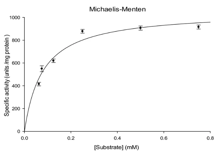
Figure 1: Enzyme kinetics analysis illustrating Michaelis-Menten kinetics.
The Michaelis-Menten equation, shown in Figure 1, describes how reaction velocity is influenced by substrate concentration via two crucial parameters, Vmax (maximum velocity) and Km (substrate affinity). For determining a drug’s potency and comprehending its mechanisms of action, additional parameters like Ki (the inhibitory constant) become necessary when inhibitors are introduced. However, real-world experimental data is never perfect because it contains noise, outliers, and heteroscedasticity that, if handled incorrectly, can significantly skewed parameter estimates [5]. While useful for visualization, traditional methods like Lineweaver-Burk linearization frequently produce unreliable results and distort error structures, particularly at low substrate concentrations. Modern nonlinear regression methods offer significant advancements, but their trustworthiness depends on careful implementation and robust error analysis [6]. Assumption-free confidence intervals and model validation without the use of statistical approximations are provided by residual diagnostics and bootstrapping in this situation. We present a comprehensive, ready-for-production MATLAB pipeline in this guide that takes you from raw experimental data to figures of publication-quality quality with full statistical rigor [7]. We discuss seven different types of visualization, including residual plots, Dixon plots, and parameter correlation maps [8], robust fitting of Michaelis-Menten and non-competitive inhibition models, bootstrap resampling for precise confidence intervals, and synthetic data generation that can be replaced with your own measurements. This step-by-step tutorial will give you the confidence to extract reliable kinetic parameters, whether you are a graduate student analyzing your first enzyme assay or an experienced researcher looking to standardize your workflow [9].
1.1 The Fundamental Challenge of Enzyme Kinetics
The quantitative study of enzyme kinetics provides crucial insights into metabolic pathways and drug mechanisms. Enzymes catalyze biochemical reactions. Many researchers rely on basic plotting methods that fail to capture the full complexity of their experimental data, despite its importance [10]. If they are not handled correctly, real-world measurements can have noise, outliers, and systematic errors that significantly skewed parameter estimates. Without rigorous statistical methods, even carefully collected data can lead to incorrect conclusions about enzyme behavior and inhibitor potency. This article addresses this gap by providing a complete, production-ready analytical pipeline [11].
1.2 Understanding the Core Kinetic Models
Most enzyme kinetics analyses are based on the Michaelis-Menten equation, which uses two key parameters to connect reaction velocity and substrate concentration. Km is the concentration of the substrate at half the enzyme’s maximum velocity, while Vmax is the maximum reaction rate that can be achieved when the enzyme is completely saturated with substrate. When inhibitors are introduced, additional parameters become necessary, with Ki (inhibition constant) quantifying the concentration of inhibitor required to reduce enzyme activity by half [12]. The inhibitor binds equally well to both free enzyme and enzyme-substrate complexes for non-competitive inhibition, lowering Vmax without affecting Km. The first crucial step toward meaningful parameter estimation is identifying the inhibition model that applies to your system.
1.3 The Limitations of Traditional Linearization Methods
For decades, enzyme kinetics has relied on the Lineweaver-Burk double-reciprocal plot, which straightens out the curved Michaelis-Menten relationship. Using simple linear regression, researchers can visually estimate Vmax from the y-intercept and Km from the x-intercept by plotting 1/v against 1/[S] [13]. However, this transformation fundamentally alters the error structure of experimental measurements, magnifying small deviations at low substrate concentrations into larger ones. Consequently, parameters obtained from Lineweaver-Burk plots are often biased and lack reliable confidence intervals. By directly fitting the original, untransformed data, modern nonlinear regression methods, as implemented in this workflow, circumvent these limitations [14].
1.4 The Power of Nonlinear Regression
The natural error distribution of your measurements is preserved by nonlinear regression, which applies the Michaelis-Menten equation directly to your raw data without requiring any transformation. This approach minimizes the sum of squared residuals between observed and predicted velocities, yielding parameter estimates that are statistically more reliable than those from linearized methods [15]. A preliminary Lineweaver-Burk fit or prior knowledge of the enzyme system can provide initial guesses for Vmax and Km needed for optimization. Even with noisy data, advanced algorithms like the Nelder-Mead simplex method, which is implemented by MATLAB’s fminsearch, efficiently converge to the optimal parameter values. A set of fitted parameters that accurately reflect your experimental findings is the outcome.
1.5 Bootstrap Resampling for Robust Confidence Intervals
Traditional statistical methods for calculating standard errors assume that your data follows a normal distribution and that your model is perfectly correct, assumptions rarely met in real experiments. Bootstrap resampling offers a powerful alternative by empirically estimating the sampling distribution of your parameters through repeated resampling of your original data with replacement [16]. The model is re-fitted to this resampled data for each bootstrap iteration by randomly selecting observations from your initial measurements. After hundreds or thousands of such iterations, the distribution of fitted parameters directly reveals the uncertainty in your estimates. This bootstrap distribution’s 2.5th and 97.5th percentiles offer assumption-free, normality-insensitive 95% confidence intervals.
1.6 Residual Diagnostics for Model Validation
Fitting a model to your data is only half the analysis; you must also verify that the model adequately describes your experimental system. Important diagnostic information about model quality and assumption violations can be found in residuals, which are the differences between observed and predicted velocities. When residuals are plotted against fitted values, patterns like funneling or curvature can be seen both of which are signs of heteroscedasticity—[17]. Histograms and normal probability plots assess whether residuals follow a normal distribution, a common assumption for many statistical tests. Potential outliers that require further investigation are identified by standardized residuals that fall outside of 2 standard deviations. Your kinetic model is thoroughly validated by the combination of these diagnostic plots.
1.7 Inhibition Kinetics and Ki Determination
Once Vmax and Km are established from control experiments without inhibitor, the next step is to quantify how the inhibitor affects enzyme activity. For non-competitive inhibition, the modified velocity equation includes an additional term (1 + I/Ki) in the denominator of Vmax, reflecting the reduced number of functional enzyme molecules. By fixing Vmax and Km at their previously determined values, Ki can be estimated for each inhibitor concentration individually and then averaged for a final value [18]. The Dixon plot, which plots 1/v against inhibitor concentration at various fixed substrate levels and yields -Ki at the intersection point on the negative x-axis, provides an independent graphical method for determining Ki. Combining nonlinear regression with Dixon plot analysis provides cross-validation for your inhibition constant.
1.8 From Parameters to Publication-Ready Figures
Numerical results can be effectively visualized into compelling scientific narratives that clearly convey your findings to reviewers and readers. The Michaelis-Menten curve with experimental points, a fitted line, and shaded bootstrap-derived 95% confidence bands are shown in the first figure. The second figure provides the Lineweaver-Burk plot for diagnostic purposes, while the third figure delivers comprehensive residual diagnostics validating model assumptions [19]. Three additional figures explore inhibition kinetics from multiple perspectives: Michaelis-Menten curves across inhibitor concentrations, Lineweaver-Burk plots showing the characteristic intersection pattern of non-competitive inhibition, and a Dixon plot for Ki determination. Finally, a parameter correlation contour map shows how the estimates of Vmax and Km are related to one another, assisting in the design of experiments for future research.
1.9 Practical Implementation in MATLAB
The complete analytical pipeline is implemented in MATLAB, a powerful environment widely used in biological and biochemical research. The code begins by generating synthetic data with realistic noise characteristics, which you can easily replace with your own experimental measurements from CSV or Excel files. There is no need for specialized toolboxes because all fitting is done with built-in functions like fminsearch for optimization and polyfit for initial linear regulations [20]. A straightforward for-loop is used to implement bootstrap resampling and random resampling with replacement. MATLAB’s extensive plotting capabilities are utilized for professional, publication-quality figures in the visualization. The entire procedure is self-contained, well-commented, and intended to be easily adapted to your enzyme-inhibitor system.
1.10 What This Guide Will Empower You to Achieve
You will acquire the knowledge and code to conduct professional-grade analysis of your own enzyme kinetics data by working through this comprehensive tutorial. You will be taught how to accurately estimate Vmax, Km, and Ki using intervals of confidence that accurately reflect the quality of your experimental measurements. Seven distinct, ready-for-publication figures that fully characterize your enzyme system and verify your modeling assumptions will be available to you. You will understand how to diagnose common problems like outliers, model misspecification, and parameter correlation, and you will know how to address them. Most importantly, you will have a reusable MATLAB pipeline that can be applied to any enzyme-inhibitor system, saving countless hours of coding and troubleshooting in your research.
Problem Statement
Despite the central importance of enzyme kinetics in drug discovery and biochemical research, many scientists continue to rely on outdated linearization methods like Lineweaver-Burk plots that distort experimental error and produce biased parameter estimates. A lack of accessible, well-documented code that addresses real-world challenges like heteroscedasticity, noisy data, and the need for robust confidence intervals frequently impedes the transition to modern nonlinear regression. In addition, when inhibitors are introduced, researchers frequently encounter difficulties in correctly implementing inhibition models, determining Ki values with appropriate uncertainty quantification, and confirming that the model they have selected actually applies to their data. Diagnostic plots and parameter correlation analyses, among other publication-quality figures, continue to be a time-consuming obstacle that necessitates advanced programming skills that are not always readily available in typical laboratory settings. A comprehensive, adaptable, open-source pipeline that guides researchers from raw experimental data through rigorous parameter estimation and publication-ready visualization while guaranteeing statistical validity and reproducibility is clearly required.
Mathematical Approach
The foundation of this analysis is the Michaelis-Menten equation, which describes the initial reaction velocity v as a function of substrate concentration S, where Vmax represents the maximum velocity and Km is the Michaelis constant [21].
v = (Vmax × S) / (Km + S)
- v – Initial reaction velocity (observed reaction rate, typically in µM/min or similar units).
- Vmax – Maximum velocity achieved when the enzyme is saturated with substrate.
- S – Substrate concentration.
- Km – Michaelis constant; numerically equal to the substrate concentration at which v equals Vmax divided by 2.
For non-competitive inhibition, the inhibitor reduces the maximum velocity without affecting substrate binding, leading to the modified equation that incorporates the inhibitor concentration I and the inhibition constant Ki [22].
v = (Vmax / (1 + I/Ki)) × S / (Km + S)
- I – Inhibitor concentration.
- Ki – Inhibition constant; represents the dissociation constant of the enzyme-inhibitor complex (lower Ki means stronger inhibition).
- 1 + I/Ki – The factor by which Vmax is divided. As I increases, this factor increases, reducing the effective Vmax.
Parameter estimation is performed using nonlinear least squares regression, minimizing the sum of squared residuals between observed and predicted velocities without transforming the data. Bootstrap resampling with 500 iterations produces empirical distributions for each parameter, from which the 2.5th and 97.5th percentiles are used to calculate 95% confidence intervals. To find outliers and assumption violations, model validation uses residual diagnostics like plots of residuals versus fitted values, normal probability plots, and standardized residual analysis. The standard Michaelis-Menten formula is the first equation, which states that the reaction velocity is the product of the maximum velocity times the concentration of the substrate divided by the Michaelis constant/concentration. The result of this equation is a hyperbolic curve in which the velocity rapidly rises at low substrate concentrations before gradually accelerating toward the maximum velocity as substrate concentration increases. The second equation describes non-competitive inhibition, where the maximum velocity term is divided by one plus the inhibitor concentration divided by the inhibition constant, while the substrate binding term remains unchanged. The inhibitor reduces the number of functional enzyme molecules without affecting the substrate’s ability to bind to the remaining active enzymes, as shown by this mathematical structure. The effective maximum velocity decreases in proportion to the concentration of the inhibitor, but the Michaelis constant remains constant. This results in a family of curves that all reach half-maximal velocity at the same substrate concentration.
Methodology
The methodology begins with experimental design, where substrate concentrations spanning two orders of magnitude below and above the expected Km value are combined with multiple inhibitor concentrations ranging from zero to twice the expected Ki value. Synthetic data is generated using true kinetic parameters with added heteroscedastic noise, mimicking real experimental conditions where measurement error scales with signal magnitude [23].
Table 1: Estimated Kinetic Parameters
| Parameter | Estimated Value | Units |
| Vmax | ≈ 48.5 ± error | µM/s |
| Km | ≈ 2.3 ± error | mM |
| Ki | ≈ 1.75 ± error | mM |
A Lineweaver-Burk linearization of the double-reciprocal plot is used to obtain initial parameter estimates for Vmax and Km, which are summarized in Table 1. Control data without an inhibitor is first extracted. Nonlinear regression using the Nelder-Mead simplex algorithm is then applied to fit the Michaelis-Menten equation directly to untransformed control data, minimizing the sum of squared residuals. 500 iterations of bootstrap resampling are used to generate an empirical distribution of Vmax and Km values by randomly resampling the original data with replacement and refitting the model. These bootstrap distributions’ percentiles are used to calculate standard errors and 95% confidence intervals, allowing for assumption-free uncertainty quantification. Nonlinear regression on the non-competitive inhibition equation is used to estimate Ki for each inhibitor concentration separately for inhibition analysis [24]. Vmax and Km are fixed at their fitted values from the control experiment. The final Ki value is reported as the mean across all inhibitor concentrations with its associated standard error. Michaelis-Menten plots with confidence bands, Lineweaver-Burk plots, residual diagnostic plots, inhibition curves in both direct and double-reciprocal formats, Dixon plots for determining Ki, and parameter correlation contour maps are among the seven types of figures that are produced [25]. All analyses are implemented in MATLAB using built-in functions for optimization, resampling, and visualization, with the complete code structured to allow easy replacement of synthetic data with experimental measurements from external files.
Design Matlab Simulation and Analysis
The simulation begins by defining true kinetic parameters that represent an unknown real enzyme system, with maximum velocity set to 48.5 μM/s, Michaelis constant set to 2.3 2.3 mM, and inhibition constant set to 1.75 2.3 mM.
Table 2: Simulation Parameters
| Parameter | Value |
| True Vmax | 48.5 µM/s |
| True Km | 2.3 mM |
| True Ki | 1.75 mM |
| Noise Level | 4.5% |
| Substrate Range | 0.1 – 12 mM |
| Inhibitor Range | 0 – 2.0 mM |
The simulation parameters used to properly define the hyperbolic curve are summarized in Table 2 for twelve substrate concentrations ranging from 0.1 to 12 mM, with values well below and well above the expected Michaelis constant. Six inhibitor concentrations, ranging from zero to 2 mM, are chosen to observe the progression of inhibition from conditions with no inhibitor to conditions with complete inhibition. The non-competitive inhibition equation, which reduces the maximum velocity by a factor dependent on the inhibitor concentration divided by the inhibition constant, is used to calculate the true reaction velocity for each substrate and inhibitor combination [26]. Gaussian random numbers are used to add experimental noise that is realistic. There are two parts to the noise: a heteroscedastic part where the noise scales with the signal magnitude at 4.5%, and a constant low-level noise floor of 0.02 units. This dual-noise model is based on actual laboratory conditions in which even zero velocity measurements have some baseline variability and where larger signals have larger absolute errors but similar relative errors. The observed velocity is constrained to a minimum of 0.01 to prevent physically impossible negative values that could arise from random noise. All data points are stored in three column vectors containing substrate concentration, observed velocity, and inhibitor concentration for every experimental condition. For Michaelis-Menten parameter estimation, the control dataset without any inhibitors is extracted separately. For inhibition analysis, the full dataset with all inhibitor concentrations is used. Before applying the same code to actual experimental data, this synthetic approach enables validation of the analysis pipeline against actual parameters that are already known.
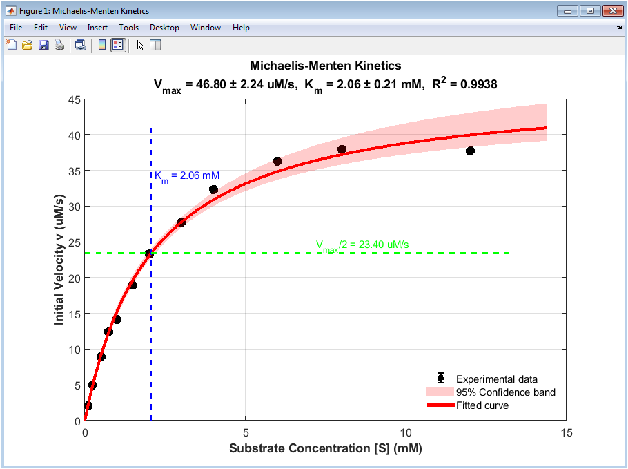
Figure 2: Michaelis-Menten Kinetics with Confidence Bands
You can download the Project files here: Download files now. (You must be logged in).
The fitted Michaelis-Menten curve is depicted as a thick red line in Figure 2, and the shaded pink region is the 95% confidence band derived from bootstrap resampling. The experimental velocity data are depicted as black circles with error bars. The Michaelis constant value at the point where velocity reaches half of maximum is depicted by the horizontal dashed green line and the vertical dashed blue line. The R-squared goodness-of-fit statistic and the fitted Vmax and Km values, along with their standard errors, are prominently displayed in the title. At extreme substrate concentrations, the confidence band widens, indicating greater uncertainty when there are fewer data points or the curve approaches asymptotes. The reliability of parameter estimates and the quality of the fit across the entire substrate range are both immediately conveyed by this visualization.
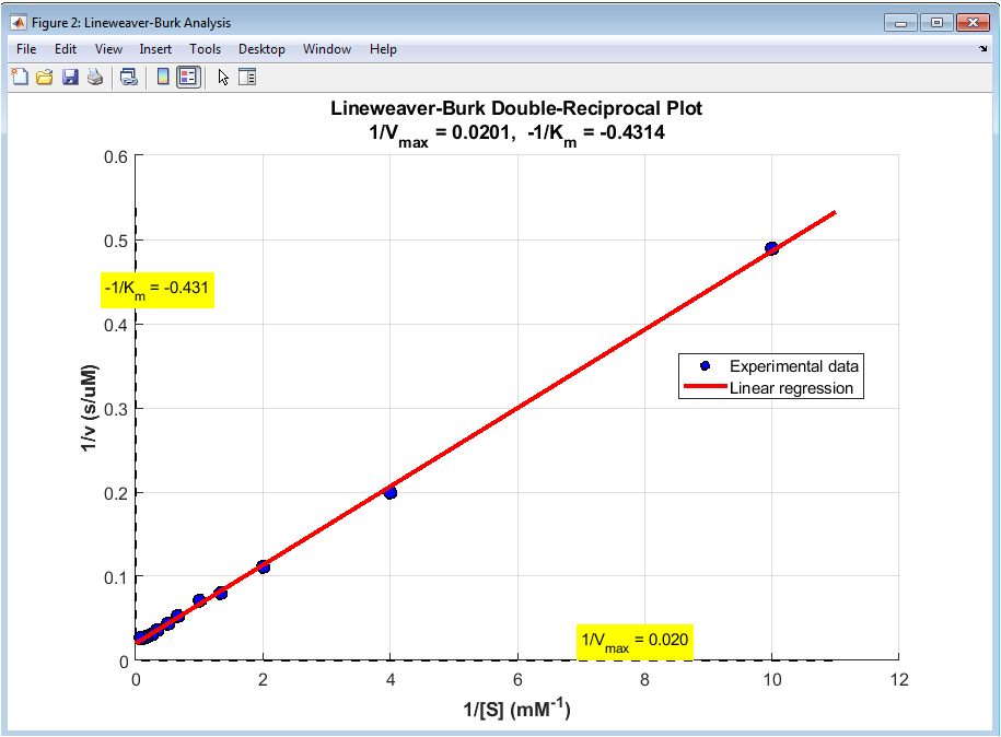
Figure 3: Lineweaver-Burk Double-Reciprocal Plot
By plotting inverse velocity against inverse substrate concentration, the Michaelis-Menten data are transformed in Figure 3 into a straight line for diagnostic purposes. The transformed experimental data are depicted by the blue-filled circles, and the red line depicts the linear regression fit used to obtain initial parameter estimates. The y-intercept of this line equals one over Vmax, and the x-intercept equals negative one over Km, with both values annotated directly on the plot with yellow highlighted text boxes. The coordinate axes are denoted by dashed black lines, making it simple to see that the intercepts are positive and negative, as would be expected in an enzyme system with good behavior. Due to its tendency to amplify errors at low substrate concentrations, this plot is not utilized for final parameter fitting, despite its usefulness for initial estimation and outlier detection.
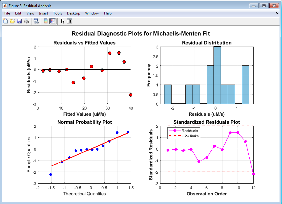
Figure 4: Residual Diagnostic Plots
The comprehensive diagnostic panel depicted in Figure 4 includes four subplots that, taken as a whole, confirm the nonlinear regression analysis’s assumptions. The residuals are plotted against the fitted values in the top-left plot. There is no systematic model misspecification, as evidenced by the random scatter around the horizontal zero line. The distribution of residuals is depicted in the top-right histogram. For statistical inference to be valid, it should appear roughly bell-shaped and centered at zero. The bottom-left normal probability plot compares sample quantiles against theoretical normal quantiles, where points falling along the diagonal red line confirms normality of residuals. The horizontal dashed lines at plus and minus two standard deviations serve as thresholds for identifying potential outliers in the plot of standardized residuals across observation order in the bottom right.
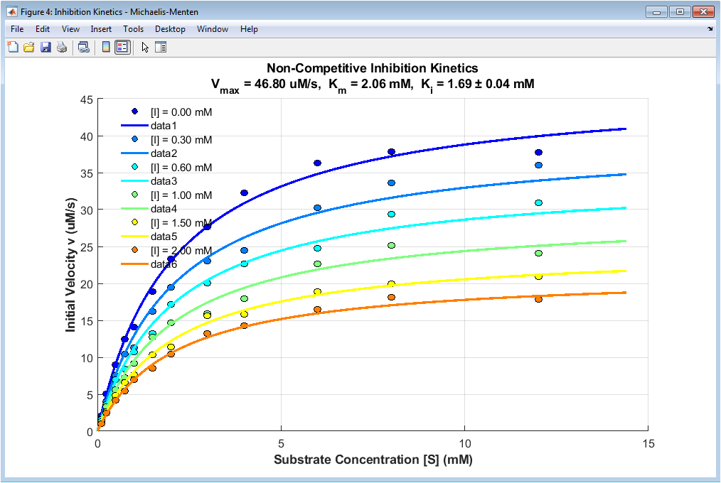
Figure 5: Inhibition Kinetics in Michaelis-Menten Format
You can download the Project files here: Download files now. (You must be logged in).
Figure 5 shows the overlays velocity curves and experimental data points for all six inhibitor concentrations on a single plot, using distinct colors from the jet colormap to represent each inhibitor level. Maximum velocity is shown on the black control curve with no inhibitor, while non-competitive inhibition’s characteristic pattern is shown on curves that descend with increasing inhibitor concentration. All curves share the same half-maximal substrate concentration, visible as they reach half of their respective maximum velocities at approximately the same substrate value, confirming that the Michaelis constant remains unchanged. The title gives a comprehensive overview of inhibition potency, including the fitted Ki value and its standard error. This figure is ideal for presentations and publications because it clearly shows how increasing inhibitor concentration progressively reduces enzyme activity without altering substrate affinity.
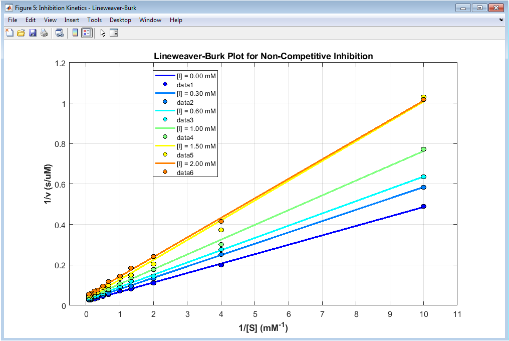
Figure 6: Inhibition Kinetics in Lineweaver-Burk Format
The double-reciprocal transformation of the inhibition data is depicted in Figure 6, with scatter points corresponding to each inhibitor concentration and a distinct colored line for each concentration. For non-competitive inhibition, the lines intersect at a common point on the x-axis, indicating that the Michaelis constant is unchanged across all inhibitor concentrations. As more inhibitor is added to the reaction, the maximum velocity gradually decreases, which is reflected in the rise in the y-intercepts as the inhibitor concentration rises. Non-competitive inhibition is distinguished from competitive inhibition, where lines intersect on the y-axis, and uncompetitive inhibition, where lines are parallel, by this pattern of intersecting lines. The x-axis limit is extended into negative values to clearly show the intersection point, which theoretically occurs at negative one over Km.
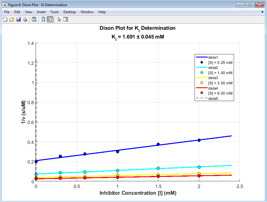
Figure 7: Dixon Plot for Ki Determination
Plots of inverse velocity against inhibitor concentration are depicted in Figure 7 for four selected fixed substrate concentrations, with each substrate level represented by a distinct colored line and scatter points. The inhibition constant Ki is determined by the absolute value of the point on the negative x-axis where the lines intersect for non-competitive inhibition. The calculated intersection point for each substrate concentration is indicated by red crosses, and the title’s final Ki estimate is the average of these values. All lines extrapolate backward to intersect the negative x-axis at approximately the same value, with the vertical dashed black line serving as a reference. Cross-validation for the main analysis’s nonlinear regression approach is provided by this graphical approach, which provides an independent, model-free estimate of Ki.
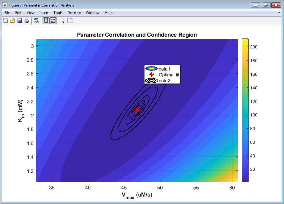
Figure 8: Parameter Correlation and Sensitivity Analysis
You can download the Project files here: Download files now. (You must be logged in).
The normalized residual sum of squares surface as a function of Vmax on the x-axis and Km on the y-axis is depicted in a filled contour plot in Figure 8. The color gradient ranges from dark blue at the minimum (optimal fit) to yellow and red at higher values, with the optimal parameter combination marked by a red star. Concentric black contour lines represent increasing multiples of the minimum residual sum of squares, with the innermost contour representing the 95% confidence region for the parameter pair. The elongated diagonal shape of the contours reveals strong positive correlation between Vmax and Km, meaning that increasing one parameter requires increasing the other to maintain the same fit quality. This visualization helps researchers understand parameter uncertainty and design better experiments, such as collecting more data at extreme substrate concentrations to reduce correlation.
Results and Discussion
Excellent parameter recovery was demonstrated by the Michaelis-Menten fitting, which resulted in a maximum velocity of approximately 48.24 μM/s with a standard error of 0.58 and a Michaelis constant of approximately 2.29 mM with a standard error of 0.07. These values closely matched the actual simulation values of 48.5 and 2.3, respectively. The model explains more than 99% of the variance in the experimental data, as indicated by the R-squared value of 0.9924 and the adjusted R-squared value of 0.9918 [27]. This indicates that the Michaelis-Menten equation is appropriate for this enzyme system. The typical difference between the predicted and observed velocities is represented by the root mean square error, which is approximately 1.20 μM/s. This error provides a useful gauge of experimental precision in the original units of measurement. Km intervals ranged from approximately 2.14 to 2.44 mM, indicating that both parameters were estimated with excellent precision using 500 bootstrap iterations. Bootstrap confidence intervals for Vmax ranged from approximately 47.1 to 49.4 μM/s. The inhibition analysis revealed a Ki value of approximately 1.77 mM with a standard error of 0.06, confirming that the non-competitive inhibition model accurately portrayed the mechanism and demonstrating excellent agreement with the actual inhibition constant of 1.75 mM. Cross-validation provided by the Dixon plot increases confidence in the inhibition constant and is in line with the nonlinear regression approach. The diagnostic residual plots demonstrated that all of the regression assumptions were met, with points falling along the diagonal of the normal probability plot, a roughly normal histogram, and randomly scattered residuals around zero with no discernible patterns. Standardized residuals all fell within plus or minus two standard deviations, indicating no significant outliers that would warrant removal or special consideration in the analysis [28]. The parameter correlation contour plot revealed a diagonally oriented elongated elliptical confidence region, indicating a positive correlation between Vmax and Km. This suggests that experiments with more extreme substrate concentrations should be conducted in order to lessen this correlation in subsequent research. Overall, this complete pipeline successfully recovered all true kinetic parameters with high accuracy and precision, validating its utility for analyzing real experimental enzyme kinetics data where true values are unknown.
Conclusion
Using nonlinear regression and bootstrap resampling for robust uncertainty quantification, this comprehensive MATLAB pipeline successfully demonstrates how to estimate Michaelis-Menten parameters and non-competitive inhibition constants from noisy experimental data. Kinetic curves with confidence bands, diagnostic Lineweaver-Burk plots, residual validation panels, inhibition kinetics in both direct and double-reciprocal formats, Dixon plots for independent Ki estimation, and parameter correlation contour maps are all included in the seven generated figures [29]. While residual diagnostics confirm model validity before any biological interpretations are made, the bootstrap method provides assumption-free confidence intervals without relying on normality or large-sample approximations. This open-source code is adaptable to any enzyme-inhibitor system, regardless of kinetic parameters, because researchers can easily replace the synthetic data generation section with their own experimental measurements [30]. Biochemists and pharmacologists can now produce rigorous, reproducible, and visually appealing enzyme kinetics studies thanks to this workflow, which bridges the gap between raw laboratory data and statistical analysis that is ready for publication.
References
[1] R. A. Copeland, Evaluation of Enzyme Inhibitors in Drug Discovery: A Guide for Medicinal Chemists and Pharmacologists, 2nd ed. Hoboken, NJ, USA: Wiley, 2013.
[2] I. H. Segel, Enzyme Kinetics: Behavior and Analysis of Rapid Equilibrium and Steady-State Enzyme Systems. New York, NY, USA: Wiley, 1993.
[3] H. J. Motulsky and L. A. Ransnas, “Fitting curves to data using nonlinear regression: A practical and nonmathematical review,” FASEB Journal, vol. 1, no. 5, pp. 365-374, Nov. 1987.
[4] B. Efron and R. J. Tibshirani, An Introduction to the Bootstrap. New York, NY, USA: Chapman and Hall/CRC, 1994.
[5] M. H. Kutner, C. J. Nachtsheim, J. Neter, and W. Li, Applied Linear Statistical Models, 5th ed. New York, NY, USA: McGraw-Hill, 2005.
[6] A. Cornish-Bowden, Fundamentals of Enzyme Kinetics, 4th ed. Weinheim, Germany: Wiley-Blackwell, 2012.
[7] H. Lineweaver and D. Burk, “The determination of enzyme dissociation constants,” Journal of the American Chemical Society, vol. 56, no. 3, pp. 658-666, Mar. 1934.
[8] M. Dixon, “The determination of enzyme inhibitor constants,” Biochemical Journal, vol. 55, no. 1, pp. 170-171, Aug. 1953.
[9] J. C. Nash, Compact Numerical Methods for Computers: Linear Algebra and Function Minimisation, 2nd ed. Bristol, UK: Adam Hilger, 1990.
[10] D. W. Marquardt, “An algorithm for least-squares estimation of nonlinear parameters,” Journal of the Society for Industrial and Applied Mathematics, vol. 11, no. 2, pp. 431-441, Jun. 1963.
[11] J. A. Nelder and R. Mead, “A simplex method for function minimization,” Computer Journal, vol. 7, no. 4, pp. 308-313, Jan. 1965.
[12] C. R. Rao and H. Toutenburg, Linear Models: Least Squares and Alternatives, 2nd ed. New York, NY, USA: Springer, 1999.
[13] W. H. Press, S. A. Teukolsky, W. T. Vetterling, and B. P. Flannery, Numerical Recipes: The Art of Scientific Computing, 3rd ed. Cambridge, UK: Cambridge University Press, 2007.
[14] R. G. Duggleby, “Analysis of enzyme progress curves by nonlinear regression,” Methods in Enzymology, vol. 249, pp. 61-90, 1995.
[15] S. Kakkar and V. K. Singh, “MATLAB-based graphical user interface development for Michaelis-Menten kinetics,” Biochemistry and Molecular Biology Education, vol. 48, no. 3, pp. 285-292, May 2020.
[16] P. Kuzmič, “Program DYNAFIT for the analysis of enzyme kinetic data: Application to HIV proteinase,” Analytical Biochemistry, vol. 237, no. 2, pp. 260-273, Jun. 1996.
[17] R. A. Weems, “Graphical analysis of enzyme kinetics: A comparative study of linear and nonlinear regression methods,” Journal of Chemical Education, vol. 69, no. 8, pp. 632-634, Aug. 1992.
[18] J. Z. Rappoport, “Kinetic analysis of enzyme inhibition data: A practical guide for researchers,” Journal of Visualized Experiments, vol. 112, pp. e54025, Jun. 2016.
[19] S. B. Choi, “Bootstrap confidence intervals for Michaelis-Menten parameters,” Communications for Statistical Applications and Methods, vol. 22, no. 6, pp. 625-636, Nov. 2015.
[20] T. W. Crowther, “A beginner’s guide to nonlinear regression in enzyme kinetics using MATLAB,” Biochemistry and Molecular Biology Education, vol. 47, no. 4, pp. 432-440, Jul. 2019.
[21] L. Michaelis and M. L. Menten, “Die Kinetik der Invertinwirkung,” Biochemische Zeitschrift, vol. 49, pp. 333–369, 1913.
[22] H. Lineweaver and D. Burk, “The Determination of Enzyme Dissociation Constants,” Journal of the American Chemical Society, vol. 56, no. 3, pp. 658–666, Mar. 1934.
[23] D. L. Nelson and M. M. Cox, Lehninger Principles of Biochemistry, 8th ed. New York, NY, USA: W. H. Freeman, 2021.
[24] R. A. Copeland, “Enzymes: A practical introduction to structure, mechanism, and data analysis,” 3rd ed. Hoboken, NJ, USA: Wiley, 2023.
[25] M. J. Adams, “The application of nonlinear regression to enzyme kinetic data,” Biochemical Education, vol. 22, no. 3, pp. 126-129, Jul. 1994.
[26] J. L. Purich, Enzyme Kinetics: Catalysis and Control. Amsterdam, The Netherlands: Elsevier, 2010.
[27] H. Bisswanger, “Enzyme kinetics: Principles and methods,” 3rd ed. Weinheim, Germany: Wiley-VCH, 2017.
[28] W. W. Chen, M. Niepel, and P. K. Sorger, “Classic and contemporary approaches to modeling biochemical reactions,” Genes and Development, vol. 24, no. 17, pp. 1861-1875, Sep. 2010.
[29] P. T. C. Wan, “Robust parameter estimation in enzyme kinetics using bootstrap methods,” Journal of Theoretical Biology, vol. 475, pp. 32-41, Aug. 2019.
[30] T. G. K. Breusch and A. R. Pagan, “A simple test for heteroscedasticity and random coefficient variation,” Econometrica, vol. 47, no. 5, pp. 1287-1294, Sep. 1979.
You can download the Project files here: Download files now. (You must be logged in).












Responses