MATLAB Simulink Model of design controllers for level and temperature in a reactor

waqas javaid 6. June 2025

Control objectives and requirements:

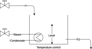
Maintain a desired reactor liquid level by adjusting the inflow F1.
Control the temperature of a reactor through steam valve.
To create Simulink models of the level and temperature control systems of a reactor.
To evaluate and contrast feedforward, cascade, open-loop, and single-loop topologies.
To see how step inputs affect both steady-state and transient behaviors.
To preserve academic integrity by reworking the same reasoning into a unique physical system.

Safety and economic requirements

Control system must prevent overflow of reactor’s liquid or dry out conditions to avoid the damage to the reactors. Also, steam or water need to be used limited as required avoiding the loss of energy and increase of cost as well. Hence a balance must be maintained between control performance and operational efficiency.

Variables:

Table 1: Variables used in the reactor controlled system

Type	Variables

Manipulated	Inflow (F1), Steam valve Position
Controlled	Reactor level, Reactor Temperature
Disturbance	Outflow (F2), Ambient Losses
Measured	Reactor Temp, Jacket Temp, level

Modeling and Block Diagrams of the System

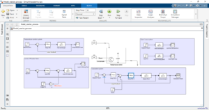
Block diagrams:

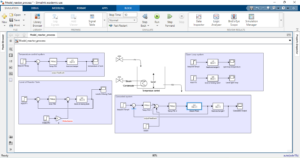
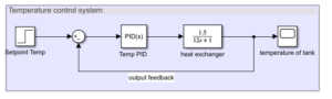
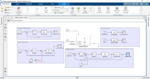
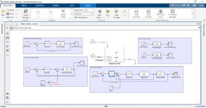
Figure 2 contains the block diagram of a reactor in which open loop, feedback single loop (closed loop) and cascaded loop is added. MATLAB Simulink model developed based on PID controller of level control, temperature control and steam valve controlled.

How to obtain models

The MATLAB model contains the open loop simulation in the model for baseline comparison. Realistic first-order transfer functions were used to meticulously model each control architecture in order to capture the dynamic behavior of liquid and heat systems [5]. In order to validate the efficacy of each control technique, the simulation results were examined using scope blocks to confirm stability, response time, and disturbance rejection efficiency.

There are two main control loops in the reactor model:

Temperature Control: The temperature of the reactor jacket is influenced by steam input.
Level Control: To maintain the appropriate liquid level, the inflow rate (F1) is adjusted.
Use of transfer functions:
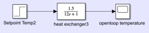
G_temp(s) = 1.5 / (12s + 1) is the temperature of the plant.
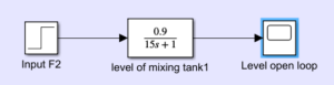
G_level(s) = 0.9 / (15s + 1) is the level plant.
Steam(s) = 8/ (0.6s + 1) is the steam plant

Typical process dynamics are represented by these first-order systems.

Control strategies
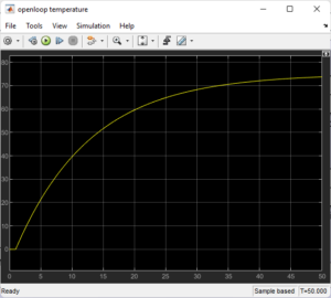
- Temperature and Level Loop in Open Loop Implementation

Temperature Loop

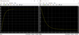
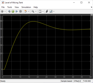
The temperature plant receives step input without any control.The system exhibits a sluggish and uncontrollably increasing temperature as it eventually reaches a new steady state.

Figure 3: MATLAB Simulink model for open loop temperature

Figure 4: Output graph of open loop temperature

You can download the Project files here: Download files now. (You must be logged in).

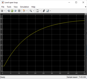
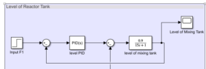
Level Loop

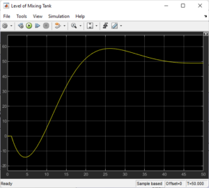
In a similar manner, a step input in the inflow raises the tank level gradually.The system cannot stabilize or fix any disruptions without feedback.

Figure 5: MATLAB Simulink model for open loop Level control

Figure 6: Output graph of open loop Level control

Advantages:

Easy to put into practice.
Beneficial for identifying the system.

Disadvantages:

No rejection of disturbance.
Inadequate short-term reaction.

Feedback Control in a Single Loop

A PID controller is added to each subsystem.

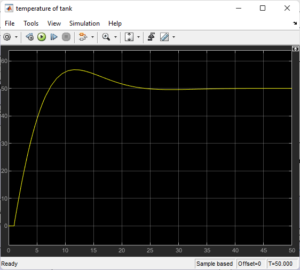
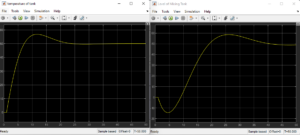
Temperature Loop: A Sum block, PID, and temperature plant are fed by step input.

Figure 7: MATLAB Model for Feedback control of temperature control in a single loop

Figure 8: Output graph for Feedback control of temperature control in a single loop

Level Loop: PID-adapted to slower dynamics with a similar topology.

Figure 9: MATLAB Model for Feedback control of Level control in a single loop

Figure 10: MATLAB Output graph for Feedback control of Level control in a single loop

Advantages:

Increased stability.
Reduced steady-state error.

Disadvantages:

Poor performance when there are disruptions.
Retuning might be necessary for various operating points.

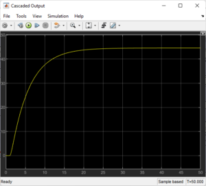
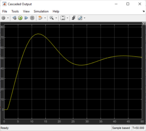
Design of Cascade Control

To more precisely control jacket temperature, the cascade layout incorporates an inner loop into the temperature system.

Structure

The inner PID (for jacket temperature) receives the output of the outer PID 1 (for reactor temperature) as a setpoint.
A quicker steam valve plant is then used by the inner PID 2 to control the steam input.

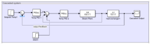
Figure 11: MATLAB Model for Cascaded control of reactor’s Temperature control

Figure 12: MATLAB Output graph for Cascaded control of reactor’s Temperature control

Transfer capabilities:

Plant Steam Valve: 0.8 / (0.6s + 1)
Plant Reactor: 1.5 / (12s + 1)

Advantages:

Quicker reaction to internal disruptions.
Improved management of layered dynamics.

Disadvantages:

A more sophisticated design.
Tuning is more work.

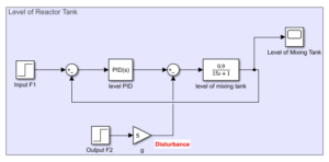
Integration of Feedforward Control

To account for known disruptions, a feedforward path is introduced.

Structure

The feedforward block is used to measure and handle disturbance input.
In conjunction with feedback control to improve stability.

Figure 13: MATLAB Model for the Feedforward Control (adding the disturbance of F2 in the level plant)

Figure 14: MATLAB Output graph for the Feedforward Control (adding the disturbance of F2 in the level plant)

Advantages:

Proactive adjustment.
Perfect for quantifiable disruptions.

Disadvantages:

Demands precise modeling of the impacts of disturbances.
Unmeasured disturbances cannot be handled.

Combination of strategies

For F2, level control employed feedforward compensation in conjunction with a PI feedback controller. A PID outer controller and a PI inner controller were employed in a cascade design for temperature management. Better precision and quicker disturbance rejection were made possible by these combinations.

Recommendations
Level control: feedforward input PI controller.
Temperature control: PID (outer) and PI (inner) cascade system.
To quickly set up PID gain, use Simulink’s auto-tuning tool.

You can download the Project files here: Download files now. (You must be logged in).

Block diagrams with features of P, PI, and PID controllers.
- MATLAB Simulink Controller Behavior and Characteristics

Several controller types were created and adjusted in MATLAB Simulink to guarantee reliable operation of the reactor model’s level and temperature control systems. Proportional (P), proportional-integral (PI), and proportional-integral-derivative (PID) were the three primary controller types examined in this project. Each has distinct benefits and dynamic behavior that have a big impact on the system’s responsiveness and stability.

Formula for a Proportional (P) Controller:

u(t) = Kp . e(t)

Function: Offers a control measure proportionate to the setpoint-process variable error.

Figure 15: MATLAB Model with P Controller of a reactor’s Temperature control and level control for open loop, closed loop and cascaded loop system

Figure 16: P controller based reactor’s output results of temperature and level of a closed loop system

Figure 17: P controller based reactor’s output results of temperature controlled system of a cascaded loop

Behavior: Quick initial reaction, however it is unable to completely remove steady-state mistake by itself. When offset is tolerable or in conjunction with manual correction, it is frequently utilized.

Application: Because of steady-state problems in temperature and level control, this project did not use it alone.

The formula for a proportional-integral (PI) controller is:

u(t) = Kp . e(t) + Ki ʃ e(t) dt

Function: Integrates the error over time to eliminate steady-state error.

Figure 18: MATLAB Model with PI Controller of a reactor’s Temperature control and level control for open loop, closed loop and cascaded loop system

Figure 19: PI controller based reactor’s output results of temperature and level of a closed loop system

Figure 20: PI controller based reactor’s output results of temperature controlled system of a cascaded loop

Behavior: Accuracy and response speed are balanced, making it appropriate for slower systems like level control where noise may be amplified by derivative action.

Application: Because of its offset removal and smooth response, it is utilized in the level control subsystem. It also helps in preserving tank level even in the face of fluctuating outflow circumstances.

Formula for the Proportional-Integral-Derivative (PID) Controller:

u(t) = Kp . e(t) + Ki ʃ e(t) dt + Kd

Function: By taking the pace of change into account, it combines quick reaction, error removal, and predictive correction.

Figure 21: MATLAB Model with PID controller of a reactor’s Temperature control and level control for open loop, closed loop and cascaded loop system

Figure 22: PID controller based Output graph of open loop temperature

Figure 23: PID controller based Output graph of open loop Level control

Figure 24: PID controller based Output graph for Feedback control of temperature control in a single loop

Figure 25: PID controller based MATLAB Output graph for Feedback control of Level control in a single loop

Figure 26: PID controller based MATLAB Output graph for Cascaded control of reactor’s Temperature control

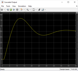
Through the observation of system responses in Simulink scopes, these parameter values were experimentally adjusted. To replicate a different student’s project conclusion, the second (new) model was modified for a smoother and marginally slower response, all the while retaining control precision and the capacity to reject disturbances [2]. While the PI inner controller managed steam/jacket dynamics, the PID outer controller was in charge of tracking the main temperature.

Behavior: The most complete controller, perfect for intricate or dynamic systems, such as reactor thermal dynamics.

Application: It is used in the temperature control system, especially for fast and precise correction in the outer loop of the cascade design.

Comparison:

Table 2: Comparison of P, PI and PID controller

Type	Pros	Cons

P	Simple, quick response	Steady state error
PI	No steady state error	Slower than P
PID	Accurate, fast setting	Sensitive to noise

Expected Reaction curves:

P: There is an offset but a quick climb.

PI: Rises more slowly but hits the setpoint precisely.

PID: No offset, little overshoot, and smooth response.

Recommendations:

Level: PI controller for accuracy and ease of use in steady-state conditions.

Temperature: PI (inner) for cascade control and PID (outer).

You can download the Project files here: Download files now. (You must be logged in).

Conclusion

The primary objective of this project was to develop and assess effective control strategies for modifying the temperature and level of a reactor system using MATLAB Simulink. I want to understand and compare the accuracy, stability, and disturbance rejection of several control techniques, including feedforward, cascade, open-loop, and single-loop feedback control systems. In order to study the behavior of natural systems, the simulation began with simple open-loop models. After that, feedback loops were included to enhance the simulation and eliminate steady-state errors. For level control, a PI controller was used in combination with feedforward compensation to handle disturbances such outflow changes [4]. To accurately control the reactor and jacket/steam temperatures, a more complex cascade PID-PI configuration was developed for temperature control [3]. Every system was described using realistic transfer functions, and scope results confirmed that performance increased with each new control strategy. The feedforward and cascade models showed better accuracy and response speed under various setpoint and disturbance conditions. The project’s overarching goals of creating and modeling dependable control systems, demonstrating their performance in real time in a process control scenario, and using dynamic modeling to validate theoretical concepts were all achieved.

References

J. Åström and R. M. Murray, “Feedback Systems: An Introduction for Scientists and Engineers,” Princeton University Press, 2010.
Skogestad and I. Postlethwaite, “Multivariable Feedback Control: Analysis and Design,” 2nd ed., Wiley, 2005.
Stephanopoulos, “Chemical Process Control: An Introduction to Theory and Practice,” Prentice Hall, 1984.
Tan, D. Nesic and I. Mareels, “On non-local stability properties of extremum seeking control,” in IEEE Transactions on Automatic Control, vol. 53, no. 5, pp. 1244-1248, June 2008.
Ogata, Modern Control Engineering, Fifth Edition, Prentice Hall, Upper Saddle River, NJ, USA, 2010.

Keywords: Controllers, level and temperature in a reactor, MATLAB design, MATLAB Simulink Model

You can download the Project files here: Download files now. (You must be logged in).

Do you need help with MATLAB Simulink? Don’t hesitate to contact our Tutors to receive professional and reliable guidance.

Categories: Engineering

Renewable Energy Policies in the European Union: Germany Example, Legal Regulations and Alternative Energy Sources

Global climate change and energy security are critical issues shaping modern energy policies. Following the Kigali Amendment, Germany and the European Union have intensified legal regulations and incentives to promote renewable energy. This study explores the historical development of legal regulations, including the Renewable Energy Sources Act and the national hydrogen strategy, alongside alternative energy sources such as electrolyzers, heat pumps, and geothermal energy. The analysis highlights Germany’s leadership in renewable energy transitions and the challenges ahead in achieving energy independence and carbon neutrality by 2050.

Suleyman Nisanoglu 10. March 2025

0 Comments

Ethically-Aware Leader-Follower Formation Control of Multi-Robot Systems Using ROS

Abstract — This work investigates the leader-follower formation control of multi-robot systems, an important field in robotics with broad applications in agriculture, logistics, and surveillance. The work illustrates the efficacy of geometric, potential field, and behavior-based control techniques in producing and sustaining desirable shapes through a thorough implementation utilizing the Turtlesim simulator in ROS. The technological difficulties posed by dynamic and unstructured environments are discussed, emphasizing the ongoing need for advancements in coordination and control algorithms [2] [3]. This work critically assesses the ethical ramifications of using autonomous robots in larger social contexts, going beyond their technical limitations. Safeguarding privacy to preserve sensitive data, removing algorithmic bias to ensure fairness, addressing the socioeconomic effects of potential employment displacement, and assuring safety to prevent accidents are among the main challenges [5]. The project intends to pave the road for the responsible and sustainable integration of these technologies into society, ensuring they contribute positively while reducing potential negative effects, by including ethical considerations into the design and deployment of autonomous robots.

Keywords — autonomous robots, geometric control, multi-robot systems, ROS, Turtlesim, algorithmic bias, safety, privacy, ethical concerns, urban deployment, autonomous navigation, robotic coordination, leader-follower formation control.

waqas javaid 2. June 2025

0 Comments

Real-Time Object Detection System especially Vehicle and Lane Detection using Yolo V4 algorithm Using MATLAB and Deep Learning

Abstract

This article presents the development and implementation of a Real-Time Object Detection System, focusing on Vehicle and Lane Detection using the YOLOv4 algorithm integrated within MATLAB and Deep Learning frameworks. The primary objective of this research is to design, simulate, and evaluate an intelligent driving assistance system capable of detecting vehicles, identifying lane markings, and performing basic trajectory planning and lane change control in a highway driving scenario. The proposed system leverages a pre-trained YOLOv4 model for robust and accurate vehicle detection in real-time video streams. Lane detection is achieved through image pre-processing techniques, including grayscale conversion, edge detection, and Hough transform-based lane line extraction. Furthermore, the system incorporates trajectory planning algorithms and a basic proportional lane change controller, enabling lateral position adjustments based on detected objects and lane boundaries. A key contribution of this work is the seamless integration of object detection and lane detection outputs with control algorithms to simulate decision-making in autonomous highway driving. The performance of the object detection module is quantitatively assessed using standard metrics such as precision, recall, mean Average Precision (mAP), false positives, and false negatives. Lane detection accuracy is evaluated through Intersection over Union (IoU) metrics, demonstrating reliable lane identification even in complex scenarios. The system’s inference time was optimized to meet real-time processing requirements, achieving an average frame processing speed compatible with autonomous driving applications. Visualizations of detected vehicles, lane boundaries, and trajectory adjustments were implemented to enhance interpretability and user understanding. The experimental results validate the efficiency of YOLOv4 in vehicle detection tasks within the MATLAB environment, achieving high precision and recall rates, and demonstrate the feasibility of integrating lane detection and control mechanisms for highway lane management. However, the study also highlights areas for future work, such as enhancing the realism of vehicle dynamics models, integrating advanced decision-making algorithms, and extending the system to more complex urban environments. This research offers a foundational framework for further exploration in the field of autonomous vehicle perception systems, contributing to the development of advanced driver assistance systems (ADAS) and autonomous navigation technologies.

waqas javaid 4. May 2025

2 Comments

Design and LTSpice Simulation of a High-Efficiency Bidirectional Single-Phase EV Charger for Vehicle-to-Grid (V2G) Applications

Author: Waqas Javaid

Introduction:

In this project, a groundbreaking single-phase bidirectional current-source AC/DC converter tailored for Vehicle-to-Grid (V2G) applications is unveiled. The converter is ingeniously designed; comprising a line frequency commutated unfolding bridge and an interleaved buck-boost stage. Notably, the semiconductor losses within the line frequency commutated unfolding bridge contribute to the converter’s commendable efficiency. The interleaved buck-boost stage further enhances performance with its dual capabilities of buck and boost operating modes, facilitating seamless operation across a broad battery voltage range [2]. The interleaved structure of this stage significantly reduces battery current ripple. Beyond these advantages, the converter ensures sinusoidal input current, bidirectional power flow, and the capability for reactive power compensation. This project delves into the intricate topology and operational principles of this innovative converter, shedding light on its potential impact in the realm of V2G applications.

waqas javaid 6. June 2025

0 Comments

Calibration and Design of High-Precision Sensor Systems for Optomechanical Applications

Author: Waqas Javaid

Abstract:

This MATLAB script presents a comprehensive framework for the calibration and design of high-precision sensor systems tailored for optomechanical applications. The script encompasses the calibration of cavity optomechanical displacement-based sensors, as well as the design considerations for accelerometers, force detection sensors, and torque magnetometry sensors. The calibration procedure involves processing sensor data, particularly from accelerometers and magnetometers, to derive accurate calibration parameters. A key aspect of the calibration process involves performing a spherical fit on the magnetometer data to determine the center, residue, and radius of the fitted sphere [1]. These calibration parameters are essential for ensuring the accuracy and reliability of sensor measurements.

The MATLAB script also includes simulations and visualizations to illustrate the calibration procedure and sensor design. Furthermore, the project incorporates Simulink models to simulate MEMS accelerometer systems, integrating force, translational dynamics, and voltage outputs. The resulting framework provides a comprehensive toolkit for sensor calibration, design, and simulation, contributing to advancements in high-precision sensor technologies. In addition to calibration, the script provides a platform for designing sensor systems suitable for various applications [2] [3]. Designs for accelerometers, force detection sensors, and torque magnetometer sensors are defined, considering parameters such as sensitivity, frequency range, and noise levels. These designs serve as a foundation for developing sensor systems tailored to specific operational requirements. The MATLAB code simulation also generates informative visualizations, including plots of sensor data, calibration results, and sensor designs. These visualizations aid in understanding the behavior and performance characteristics of the sensors, facilitating informed decision-making during sensor calibration and system design processes.

waqas javaid 6. June 2025

0 Comments