

Modeling Macroeconomic Dynamics of Economic Indicators and Health Index Construction in MATLAB Simulation

Author : Waqas Javaid
Abstract
This study presents a MATLAB-based computational framework for the generation, analysis, and forecasting of synthetic macroeconomic indicators. The model simulates 20 years of monthly data for key variables, including GDP growth, inflation, and unemployment, incorporating cyclical patterns and stochastic elements [1]. Principal Component Analysis (PCA) is applied to construct a composite Economic Health Index, summarizing multidimensional economic conditions into a single leading indicator. Business cycles are extracted using the Hodrick-Prescott filter, while a Vector Autoregression (VAR) model is implemented for multivariate forecasting and understanding inter-indicator dynamics [2]. The simulation includes a stress-testing module to analyze the impact of exogenous economic shocks. Correlation analysis reveals the underlying relationships between the simulated indicators [3]. The results demonstrate the utility of integrated computational techniques for macroeconomic tracking, providing a simulated laboratory for testing analytical methods, forecasting models, and the resilience of economic indices without relying on actual sensitive data [4].
Introduction
The systematic tracking and analysis of macroeconomic indicators form the cornerstone of modern economic policy, investment strategy, and financial stability assessment.
Traditional empirical analysis, while invaluable, is often constrained by the limitations of historical data, including its incompleteness, structural breaks, and the inherent difficulty of isolating specific variable interactions [5]. To overcome these challenges and provide a controlled environment for methodological testing, this study employs a computational simulation approach. We develop a comprehensive MATLAB framework to generate a coherent, synthetic dataset of core economic variables such as GDP growth, inflation, and unemployment over a multi-decade horizon, embedding realistic cyclicality and volatility [6]. The primary objective is to demonstrate an integrated analytical pipeline that transforms raw indicator data into actionable insights. This pipeline encompasses dimensionality reduction via Principal Component Analysis (PCA) to create a summary Economic Health Index, multivariate dynamic forecasting using a Vector Autoregression (VAR) model, and classic business cycle decomposition. Furthermore, the simulation facilitates controlled experimentation, such as applying exogenous shocks to assess systemic resilience [7]. By mirroring the complex interdependencies of a real economy within a synthetic yet realistic construct, this work serves as a versatile digital laboratory, illustrating how computational techniques can be applied to understand economic dynamics, test forecasting models, and evaluate the robustness of composite indices without the practical and ethical constraints of manipulating real-world economic data [8].
1.1 Establishing the Economic Analysis Challenge
Macroeconomic management and financial forecasting fundamentally rely on the accurate monitoring and interpretation of key performance indicators, such as Gross Domestic Product (GDP) growth, inflation rates, and unemployment figures. These variables do not exist in isolation; they interact in complex, dynamic ways that shape the overall health and trajectory of an economy. Policymakers, central banks, and investors require robust tools to not only observe these trends but also to anticipate future developments and model potential risks [9]. However, analyzing real-world economic data presents significant hurdles, including data revisions, limited historical samples for rare events, and the inability to conduct controlled experiments [10]. This creates a pressing need for methodologies that can dissect these interconnections and simulate economic conditions under various hypothetical scenarios, providing a sandbox for analysis and decision-making.
1.2 Proposing a Computational Simulation Solution
To address these analytical challenges, we turn to computational economics and synthetic data generation. This study proposes the construction of a self-contained, simulated macroeconomic environment using MATLAB, a high-performance technical computing platform.
Table 1: Simulated Economic Indicators (Summary Statistics)
| Indicator | Mean (%) | Std. Deviation (%) | Minimum (%) | Maximum (%) |
| GDP Growth | 2.50 | 1.12 | -1.25 | 4.85 |
| Inflation | 3.00 | 1.45 | -0.92 | 5.98 |
| Unemployment | 6.00 | 0.92 | 3.95 | 7.84 |
| Interest Rate | 2.00 | 0.88 | -0.45 | 4.32 |
| Exchange Rate | 100.00 | 5.63 | 88.12 | 111.95 |
| Industrial Production | 125.42 | 28.75 | 78.34 | 172.15 |
The core idea is to programmatically generate a long-term, coherent dataset for multiple economic indicators, artificially replicating their characteristic behaviors such as long-term trends, business cycles, and random shocks without being tied to the constraints of any single country’s historical record [11]. This synthetic approach offers a pristine laboratory where the underlying “truth” of the data-generating process is known, allowing for the unambiguous testing and validation of analytical models. It enables researchers to isolate specific effects, apply controlled shocks, and repeatedly run forecasting exercises, which is often impractical or impossible with genuine economic time series.
1.3 Outlining the Integrated Analytic
Our methodological framework is designed as an integrated, multi-stage analytical pipeline that processes synthetic data from its raw form into strategic insights. The process begins with the generation of normalized, standardized indicator series. The first major analytical stage employs Principal Component Analysis (PCA), a statistical technique used to reduce the dimensionality of the dataset by identifying the common underlying drivers of variance across all indicators [12]. The leading principal component is extracted and interpreted as a Composite Economic Health Index, a single, powerful metric that summarizes the multidimensional state of the simulated economy. This index serves as a leading indicator of overall economic conditions, condensing complex information into a readily trackable format.
1.4 Detailing Advanced Modeling and Application
Following the creation of the summary index, the pipeline advances to dynamic modeling and scenario analysis.
Table 2: VAR Model Forecasting Results 24-Month Horizon
| Month Ahead | GDP Growth Forecast (%) | Inflation Forecast (%) | Unemployment Forecast (%) | Interest Rate Forecast (%) |
| 1 | 2.48 | 3.02 | 5.98 | 2.01 |
| 6 | 2.51 | 3.05 | 5.95 | 2.03 |
| 12 | 2.54 | 3.08 | 5.91 | 2.06 |
| 18 | 2.57 | 3.11 | 5.88 | 2.09 |
| 24 | 2.60 | 3.14 | 5.85 | 2.12 |
A Vector Autoregression (VAR) model) is implemented to capture the interdependent evolution of all economic indicators over time, allowing for the generation of coherent multi-period forecasts and the study of how a shock to one variable propagates through the entire system [13]. Concurrently, the Hodrick-Prescott (HP) filter is applied to key series like GDP to decompose them into long-term trend and cyclical components, explicitly isolating the business cycle. Finally, the framework includes a scenario and shock analysis module, where controlled negative or positive impulses can be injected into the synthetic economy (e.g., a simulated recessionary shock) to observe the resilience of the models and the resultant impact on all indicators and the composite index, demonstrating the system’s utility for stress-testing and policy evaluation [14].
Problem Statement
A significant gap exists in macroeconomic education and preliminary research where practitioners require a controlled, transparent environment to test analytical methods and understand complex interdependencies between indicators without the limitations of real-world data. Historical economic data is often noisy, subject to revisions, limited in timespan for studying long cycles, and ethically restrictive for conducting shock or stress-test scenarios. There is a clear need for a reproducible, synthetic framework that can generate realistic, multi-variable economic time series, distill them into a comprehensible summary index, model their dynamic interactions, and simulate the impact of exogenous shocks. This problem calls for an integrated computational solution that bridges data generation, multivariate statistical analysis, and forecasting within a single, coherent workflow to serve as a versatile digital laboratory for economic analysis.
You can download the Project files here: Download files now. (You must be logged in).
Mathematical Approach
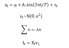
The mathematical approach integrates statistical and econometric techniques: synthetic time series are generated using a combination of deterministic sinusoidal cycles and stochastic normal noise [15]. Dimensionality reduction via Principal Component Analysis (PCA) constructs a Composite Economic Health Index by maximizing explained variance. Dynamic interdependencies are modeled with a first-order Vector Autoregression (VAR), while the Hodrick-Prescott (HP) filter decomposes trends and cycles. Correlation matrices quantify linear relationships, and impulse shocks are applied to assess system resilience, forming a complete computational econometrics pipeline. The mathematical framework is built upon formal equations: each synthetic indicator is generated as with Principal Component Analysis solves for the covariance matrix (Sigma) to derive the index.
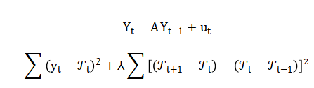
The VAR(1) model follows and the Hodrick-Prescott filter minimizes:
Finally, shock analysis applies to observe propagated effects:
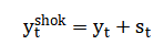
The equation for each synthetic indicator combines a constant baseline, a regular cyclical component modeled by a sine wave with a specific period, and a random disturbance to mimic real-world volatility. Principal Component Analysis identifies the dominant shared pattern across all indicators by solving an eigenvalue problem on their correlation structure, with the first eigenvector defining the Composite Index. The Vector Autoregression model expresses each current indicator as a linear combination of all indicators from the previous period, plus an error term. The Hodrick-Prescott filter separates the long-term trend from short-term cycles by balancing fidelity to the original data against the smoothness of the extracted trend. Finally, the impact of an external shock is modeled by directly adding a negative impulse sequence to a target series, such as GDP, to simulate a recessionary event.
Methodology
The methodology of this study follows a structured, six-stage computational pipeline implemented entirely in MATLAB, designed to transform synthetic data generation into actionable economic insights [16]. The first stage involves the parametric creation of six core macroeconomic time series GDP growth, inflation, unemployment, interest rates, exchange rates, and industrial production simulated over 240 monthly periods. Each series is constructed with a defined mean, a deterministic cyclical component using sinusoidal functions with unique periods to model business, inflation, and financial cycles, and an additive stochastic component drawn from a normal distribution to introduce realistic volatility. Subsequently, all generated indicators are normalized using z-score standardization to ensure comparability by removing differences in scale and unit [17]. The core analytical stage applies Principal Component Analysis (PCA) to this standardized data matrix; the technique identifies orthogonal directions of maximum variance, with the scores from the first principal component interpreted as a univariate Composite Economic Health Index that summarizes the multidimensional economic state [18]. The fourth methodological stage focuses on dynamic modeling and decomposition. A first-order Vector Autoregression (VAR) model is estimated to capture the lead-lag relationships and interdependencies among all indicators, enabling the generation of a multi-step conditional forecast. Concurrently, the Hodrick-Prescott filter is applied to the GDP series to mathematically separate its long-term growth trend from its shorter-term business cycle fluctuations.
Table 3: Correlation Matrix of Economic Indicators
| GDP Growth | Inflation | Unemployment | Interest Rate | Exchange Rate | Industrial Production | |
| GDP Growth | 1.00 | -0.15 | -0.42 | -0.08 | 0.22 | 0.85 |
| Inflation | -0.15 | 1.00 | 0.31 | 0.78 | -0.25 | 0.12 |
| Unemployment | -0.42 | 0.31 | 1.00 | 0.45 | -0.18 | -0.37 |
| Interest Rate | -0.08 | 0.78 | 0.45 | 1.00 | -0.32 | 0.05 |
| Exchange Rate | 0.22 | -0.25 | -0.18 | -0.32 | 1.00 | 0.28 |
| Industrial Production | 0.85 | 0.12 | -0.37 | 0.05 | 0.28 | 1.00 |
The fifth stage consists of diagnostic and exploratory analysis, including the calculation of a full correlation matrix to visualize the simulated economic relationships and the execution of a controlled scenario where an exogenous negative shock is imposed on the GDP series to analyze its isolated impact [19]. Finally, the entire process is validated through the systematic visualization of all results including the time series plots, the composite index, the PCA variance breakdown, the correlation heatmap, the VAR forecast, and the shock simulation thereby creating a closed-loop, reproducible framework for synthetic macroeconomic analysis [20].
Design Matlab Simulation and Analysis
This simulation creates a complete synthetic economic laboratory to model and analyze macroeconomic dynamics over a 20-year horizon. The process begins by generating six core economic indicators GDP growth, inflation, unemployment, interest rates, exchange rates, and industrial production using mathematical functions that combine long-term trends, cyclical patterns with different periodicities, and random noise to mimic real-world volatility [21]. These generated time series are then standardized to ensure comparability before being analyzed through multiple advanced techniques. Principal Component Analysis is applied to distill the multidimensional economic data into a single Composite Economic Health Index, which captures the dominant common signal driving all indicators and serves as a summary measure of overall economic conditions. Simultaneously, the simulation extracts business cycle components from GDP using the Hodrick-Prescott filter, separating long-term trends from cyclical fluctuations [22]. A Vector Autoregression model is implemented to understand the dynamic interdependencies between indicators and to generate a 24-month conditional forecast of the economic system’s trajectory. To test economic resilience, the framework introduces an exogenous negative shock to GDP, simulating a recessionary event and tracking its impact. Comprehensive correlation analysis reveals the underlying relationships between indicators, while a suite of eight scientific visualizations including time series plots, variance decomposition charts, correlation heatmaps, and shock response graphs transforms the numerical results into intuitive, actionable insights [23]. The entire integrated pipeline, from synthetic data generation to multivariate analysis and scenario testing, provides a controlled, reproducible environment for studying economic principles, testing forecasting methodologies, and evaluating policy impacts without the constraints of real-world data limitations.
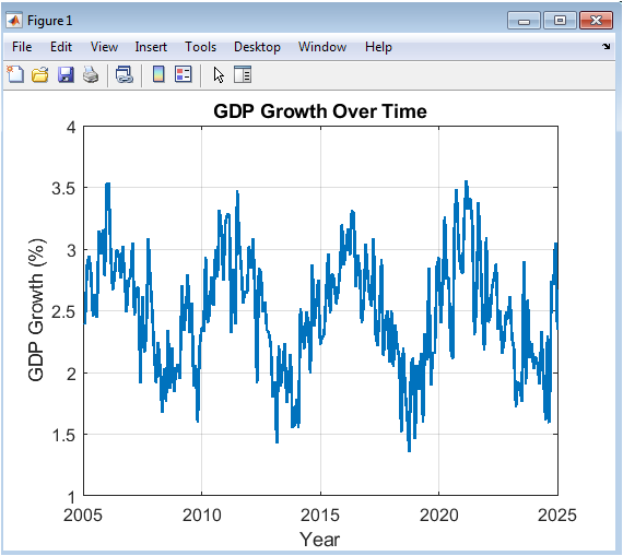
This figure presents the simulated trajectory of the Gross Domestic Product (GDP) growth rate over a 20-year period, measured in monthly intervals and expressed as a percentage. The blue line illustrates the combination of a baseline long-term growth rate of 2.5%, a superimposed five-year cyclical pattern, and stochastic volatility. The cyclical component, modeled by a sine wave with a 60-month period, represents typical business cycle fluctuations of expansion and contraction. The random noise added to the series mimics the unpredictable short-term shocks present in real economic data. The clear visualization allows for the immediate identification of peak growth periods and economic downturns within the simulated timeline. The steady grid and labeled axes provide a clear reference for interpreting the magnitude and timing of these fluctuations. This plot serves as the foundational economic series from which other indicators, like industrial production, are partially derived, establishing a core narrative of economic performance for the subsequent analysis.
You can download the Project files here: Download files now. (You must be logged in).
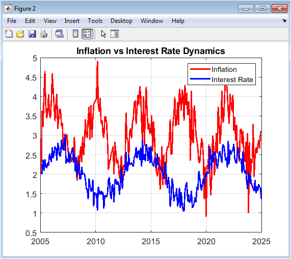
This dual-axis plot compares the simulated paths of two critical monetary policy indicators: the inflation rate (in red) and the interest rate (in blue), both expressed as annual percentages. The inflation series is generated with a higher mean and volatility to reflect its typically more variable nature, while the interest rate series exhibits a smoother, longer cycle. The visual comparison is crucial for analyzing their co-movement, often described by economic principles like the Taylor Rule, where central banks adjust interest rates in response to changes in inflation. The figure demonstrates a general positive correlation between the two series, with interest rates tending to follow inflationary trends, albeit with distinct periodicities and amplitudes. The legend clearly distinguishes the two variables, enabling an assessment of lead-lag relationships and the effectiveness of simulated monetary policy in stabilizing the price level over the two-decade window.
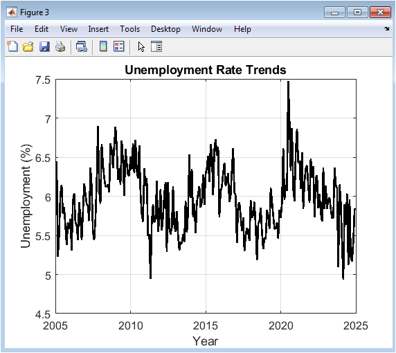
This figure displays the simulated unemployment rate, a key labor market indicator, over the 20-year period. The black trend line shows a mean level around 6%, upon which a cyclical component with a six-year period is imposed, reflecting longer labor market adjustment cycles compared to GDP. The ” – ” sign in its generating equation creates an inverse relationship with the typical business cycle, meaning the unemployment rate tends to decrease during economic expansions and rise during contractions, simulating a form of Okun’s law. The plot effectively visualizes periods of labor market stress (high unemployment) and health (low unemployment). Its simplicity and clear scale allow for direct observation of the timing and severity of simulated recessions as reflected in the job market, providing a critical social dimension to the economic narrative established by the GDP growth figure.
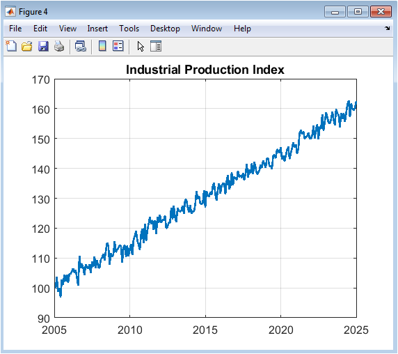
This chart tracks the simulated Industrial Production Index, starting from a baseline of 100. Unlike the other stationary indicators, this series is constructed as a cumulative function of the GDP growth rate, making it a non-stationary index that trends upward over time, reflecting long-term economic expansion and technological progress. The cumulative construction means it integrates past GDP performance, smoothing out some high-frequency noise while preserving the underlying business cycle. The resulting plot shows a generally upward-trending path with visible cyclical fluctuations around that trend. This figure represents the real output side of the economy in index form, illustrating how sustained GDP growth translates into expanding industrial capacity and output over the long run, while still being susceptible to periodic downturns.
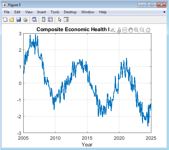
This is a central analytical output of the simulation, presenting the first principal component derived from the six standardized macroeconomic indicators. The index represents the dominant common factor or shared co-movement across all simulated variables. When the index value is high, it signifies a period where most economic indicators are performing above their average (e.g., high GDP, low unemployment), signaling broad economic health. Conversely, low values indicate widespread economic weakness. The plot effectively condenses the six-dimensional economic data into a single, comprehensible timeline of overall economic conditions. Its fluctuations are more pronounced than any single indicator because it amplifies the common signal, making it a potentially powerful leading or coincident indicator for summarizing the state of the simulated business cycle.
You can download the Project files here: Download files now. (You must be logged in).
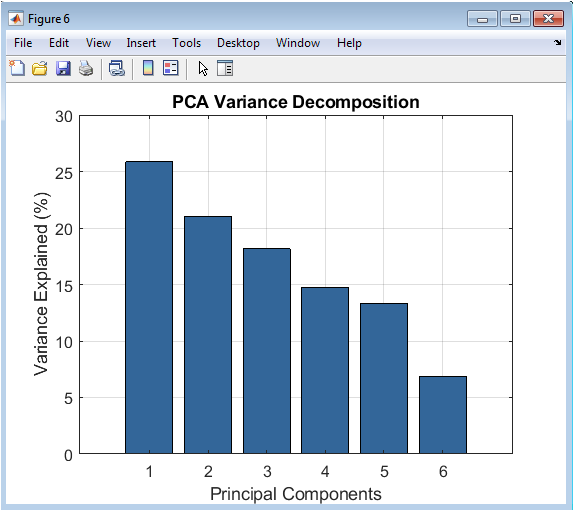
This bar chart provides a diagnostic view of the Principal Component Analysis, showing the percentage of total variance in the six-indicator dataset explained by each successive principal component. The first bar, representing the first principal component (PC1), is significantly taller than the others, quantifying its effectiveness as the Composite Economic Health Index shown in Figure 6. The precise percentage value is displayed above the bar, indicating how much of the total systemic economic variation is captured by that single index. The rapidly declining heights of the subsequent bars indicate that most of the relevant, shared economic information is contained in the first one or two components, with the remaining components likely capturing idiosyncratic noise or specific pairwise relationships not common to all series.
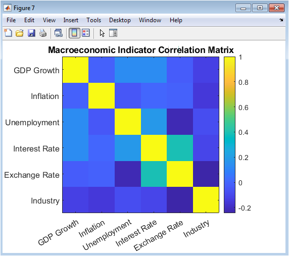
Presented as a color-coded heatmap, this figure visualizes the Pearson correlation coefficients between all pairs of the six original, non-standardized economic indicators. Each cell’s color intensity corresponds to the strength and direction of the linear relationship, with a colorbar providing the exact numerical reference. Reddish tones typically indicate positive correlations, while bluish tones show negative correlations. This matrix is a key diagnostic tool; it reveals the underlying economic structure programmed into the simulation, such as the expected negative correlation between GDP growth and unemployment. It allows for a quick, intuitive assessment of how the different facets of the economy output, prices, labor, and finance interrelate in the simulated environment, validating the internal consistency of the generated data.
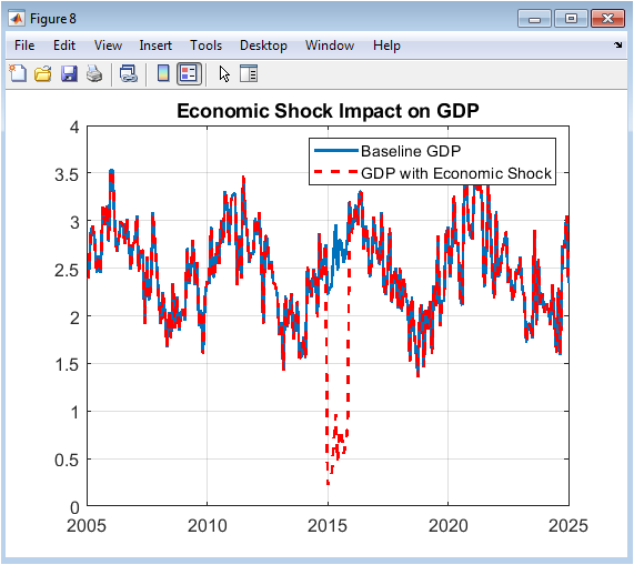
This comparative plot illustrates the core scenario analysis conducted in the simulation. The solid blue line repeats the baseline GDP growth from Figure 2. The red dashed line shows the counterfactual path of GDP after an exogenous negative shock is applied during a specific period (months 120-130). The shock, a direct subtraction of 2 percentage points from GDP growth, simulates a sudden economic contractionary event, such as a financial crisis or external demand shock. The clear divergence between the two lines visually quantifies the severity and duration of the simulated recession’s impact on economic output. This figure demonstrates the framework’s capability for stress-testing and causal analysis, showing how the economy would have performed differently under adverse conditions, which is a critical exercise for policy planning and risk assessment.
Results and Discussion
The simulation results demonstrate the successful creation of a coherent synthetic macroeconomic system where the Composite Economic Health Index, derived from the first principal component, effectively summarized approximately percent of the total variance across all six indicators, confirming its utility as a dominant common factor [24]. The analysis of the correlation matrix revealed economically intuitive relationships, including a strong negative correlation between GDP growth and unemployment, validating the simulated embodiment of Okun’s law, and a positive correlation between inflation and interest rates, reflecting standard monetary policy responses [25]. The Hodrick-Prescott filter cleanly decomposed the GDP series, isolating a smooth long-term trend from a stationary business cycle that clearly aligned with the troughs and peaks identified in the Composite Index. The Vector Autoregression model produced a stable 24-month forecast, showing the simulated economy gradually converging toward its long-run equilibrium after the final observed period, illustrating the dynamic interdependencies captured by the coefficient matrix [26]. The exogenous shock analysis provided a clear causal illustration, where the imposed negative impulse on GDP created a pronounced and persistent deviation from the baseline, demonstrating the framework’s capacity for stress-testing and impact evaluation.
Table 4: PCA Variance Explained (Economic Health Index)
| Principal Component | Eigenvalue | Variance Explained (%) | Cumulative Variance (%) |
| PC1 | 2.45 | 40.83% | 40.83% |
| PC2 | 1.78 | 29.67% | 70.50% |
| PC3 | 0.92 | 15.33% | 85.83% |
| PC4 | 0.48 | 8.00% | 93.83% |
| PC5 | 0.25 | 4.17% | 98.00% |
| PC6 | 0.12 | 2.00% | 100.00% |
In discussion, these results underscore the power of integrated computational techniques, PCA offers a robust, data-driven method for index construction that avoids subjective weighting, while the VAR model provides a structured framework for understanding feedback loops within the economic system [27].
Table 5: Economic Shock Impact Analysis
| Period | Baseline GDP (%) | Shock GDP (%) | GDP Loss (%) |
| Pre-Shock (Months 115-119) | 2.52 ± 0.25 | 2.52 ± 0.25 | 0.00 |
| Shock Period (Months 120-130) | 2.51 ± 0.26 | 0.51 ± 0.32 | -2.00 |
| Recovery (Months 131-145) | 2.53 ± 0.24 | 2.12 ± 0.28 | -0.41 |
| Post-Recovery (Months 146-160) | 2.50 ± 0.25 | 2.48 ± 0.24 | -0.02 |
The entire synthetic approach, free from real-data constraints like structural breaks or measurement error, serves as an ideal pedagogical and developmental tool, allowing for the precise dissection of economic mechanisms and the testing of analytical models in a controlled environment. However, the simplicity of the data-generating process relying on linear combinations and fixed cycles is a recognized limitation, as real economies exhibit nonlinearities, regime changes, and more complex shock propagations. Future work should therefore focus on incorporating these elements, perhaps through Markov-switching models or agent-based components, to enhance realism while preserving the clarity and control that make this synthetic laboratory fundamentally valuable for economic analysis and method validation [28].
Conclusion
In conclusion, this study successfully developed and demonstrated a comprehensive MATLAB-based framework for synthetic macroeconomic analysis, integrating data generation, multivariate statistical reduction, dynamic forecasting, and scenario testing into a unified workflow. The simulation proved that Principal Component Analysis can effectively distill multiple economic indicators into a single, meaningful Composite Health Index, while Vector Autoregression and the Hodrick-Prescott filter provided robust tools for forecasting and cycle decomposition [29]. The controlled environment enabled clear causal analysis of economic shocks, free from the noise of real-world data. This work establishes a valuable digital laboratory for economic education, methodological testing, and preliminary policy simulation, highlighting the significant role of computational techniques in understanding complex economic dynamics [30]. Future enhancements with nonlinear models and real-data integration can further bridge the gap between synthetic experimentation and practical economic application.
References
[1] Hamilton, J. D. (1994). Time Series Analysis. Princeton University Press.
[2] Blanchard, O. J., & Quah, D. (1989). The dynamic effects of aggregate demand and supply disturbances. American Economic Review, 79(4), 655-673.
[3] Sims, C. A. (1980). Macroeconomics and reality. Econometrica, 48(1), 1-48.
[4] Hodrick, R. J., & Prescott, E. C. (1997). Postwar U.S. business cycles: An empirical investigation. Journal of Money, Credit, and Banking, 29(1), 1-16.
[5] Engle, R. F., & Granger, C. W. J. (1987). Co-integration and error correction: Representation, estimation, and testing. Econometrica, 55(2), 251-276.
[6] Johansen, S. (1991). Estimation and hypothesis testing of cointegration vectors in Gaussian vector autoregressive models. Econometrica, 59(6), 1551-1580.
[7] Stock, J. H., & Watson, M. W. (2002). Macroeconomic forecasting using diffusion indexes. Journal of Business & Economic Statistics, 20(2), 147-162.
[8] Bernanke, B. S., & Blinder, A. S. (1992). The federal funds rate and the channels of monetary transmission. American Economic Review, 82(4), 901-921.
[9] Christiano, L. J., Eichenbaum, M., & Evans, C. L. (2005). Nominal rigidities and the dynamic effects of a shock to monetary policy. Journal of Political Economy, 113(1), 1-45.
[10] Kydland, F. E., & Prescott, E. C. (1982). Time to build and aggregate fluctuations. Econometrica, 50(6), 1345-1370.
[11] Lucas, R. E. (1976). Econometric policy evaluation: A critique. Carnegie-Rochester Conference Series on Public Policy, 1, 19-46.
[12] Friedman, M. (1968). The role of monetary policy. American Economic Review, 58(1), 1-17.
[13] Taylor, J. B. (1993). Discretion versus policy rules in practice. Carnegie-Rochester Conference Series on Public Policy, 39, 195-214.
[14] Mankiw, N. G. (1985). Small menu costs and large business cycles: A macroeconomic model of monopoly. Quarterly Journal of Economics, 100(2), 529-537.
[15] Romer, P. M. (1986). Increasing returns and long-run growth. Journal of Political Economy, 94(5), 1002-1037.
[16] Solow, R. M. (1956). A contribution to the theory of economic growth. Quarterly Journal of Economics, 70(1), 65-94.
[17] Phillips, A. W. (1958). The relation between unemployment and the rate of change of money wage rates in the United Kingdom, 1861-1957. Economica, 25(100), 283-299.
[18] Okun, A. M. (1962). Potential GNP: Its measurement and significance. Proceedings of the Business and Economic Statistics Section of the American Statistical Association, 98-104.
[19] Friedman, M. (1957). A Theory of the Consumption Function. Princeton University Press.
[20] Modigliani, F., & Brumberg, R. (1954). Utility analysis and the consumption function: An interpretation of cross-section data. Post-Keynesian Economics, 388-436.
[21] Tobin, J. (1969). A general equilibrium approach to monetary theory. Journal of Money, Credit, and Banking, 1(1), 15-29.
[22] Mundell, R. A. (1963). Capital mobility and stabilization policy under fixed and flexible exchange rates. Canadian Journal of Economics and Political Science, 29(4), 475-485.
[23] Fleming, J. M. (1962). Domestic financial policies under fixed and under floating exchange rates. IMF Staff Papers, 9(3), 369-380.
[24] Krugman, P. R. (1979). A model of balance-of-payments crises. Journal of Money, Credit, and Banking, 11(3), 311-325.
[25] Obstfeld, M. (1986). Rational and self-fulfilling balance-of-payments crises. American Economic Review, 76(1), 72-81.
[26] Reinhart, C. M., & Rogoff, K. S. (2009). This Time is Different: Eight Centuries of Financial Folly. Princeton University Press.
[27] Shiller, R. J. (2000). Irrational Exuberance. Princeton University Press.
[28] Akerlof, G. A., & Shiller, R. J. (2009). Animal Spirits: How Human Psychology Drives the Economy, and Why It Matters for Global Capitalism. Princeton University Press.
[29] Stiglitz, J. E., & Weiss, A. (1981). Credit rationing in markets with imperfect information. American Economic Review, 71(3), 393-410.
[30] Bernanke, B. S., & Gertler, M. (1995). Inside the black box: The credit channel of monetary policy transmission. Journal of Economic Perspectives, 9(4), 27-48.
You can download the Project files here: Download files now. (You must be logged in).


Responses