

Using Matlab, Environmental Control Strategies for Maximum Yield: How to Build an Automated Greenhouse

Author : Waqas Javaid
Abstract
Using PID-based control algorithms, this article presents a comprehensive framework for automating greenhouses that focuses on simultaneously controlling temperature, humidity, (CO_2) concentration, light intensity, and soil moisture. Over the course of a 24-hour period, a comprehensive simulation model that takes into account the physical dynamics of the greenhouse, disturbances from the outside weather, plant transpiration, and photosynthesis rates, are developed and examined. System effectiveness is evaluated using key performance metrics like the growth potential index, energy consumption, water use, and root mean square error (RMSE) [1]. The findings show that while optimizing resource utilization, well-tuned PID controllers keep environmental conditions close to setpoints (temperature RMSE 0.5°C, humidity RMSE 5%) [2]. Growers and engineers can use this framework to implement data-driven automation that increases crop yield, lowers operating costs, and reduces weather-related risks [3].
Introduction
Automation of greenhouses has emerged as a crucial tool for ensuring food security, resource efficiency, and consistent crop quality in modern agriculture.
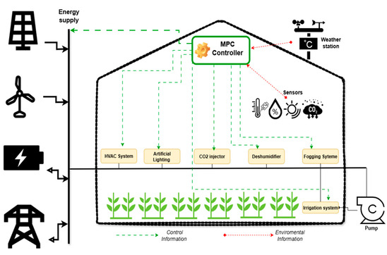
Figure 1: Smart Greenhouse Automation System Intelligent Climate, Irrigation, Lighting, and CO_2 Control for Efficient and Sustainable Plant Growth.
The days when growers managed their growing environments solely through manual thermostats, regular watering, and intuition are depicted in Figure 1. Temperature, humidity, (CO_2) levels, light intensity, and soil moisture are all continuously monitored and adjusted by sophisticated control systems in real time today [4]. However, designing such a system is difficult due to the complex interrelationships between greenhouse variables—changes in temperature affect humidity, and an increase in (CO_2) without sufficient light wastes resources [5]. This article introduces a data-driven automation framework built around PID (Proportional-Integral-Derivative) controllers, which are widely used in industrial control for their simplicity and effectiveness [6]. We incorporate realistic outdoor weather disturbances, patterns of solar radiation, and plant physiological processes like transpiration and photosynthesis into our 24-hour cycle simulation [7]. The heaters, coolers, humidifiers, dehumidifiers, (CO_2) injectors, irrigation pumps, fans, and additional LED lighting are all included in the model. We demonstrate how automation maintains optimal conditions while minimizing operational costs by analyzing important performance metrics like RMSE, energy consumption, water consumption, and growth potential [8]. This guide provides the fundamental knowledge and practical insights necessary for success whether you are a commercial grower looking to upgrade an existing facility or a hobbyist planning a smart greenhouse. Last but not least, we talk about common pitfalls like PID windup and actuator oversizing and tried-and-true ways to avoid them [9].
1.1 The Transformation of Modern Agriculture
The dual pressures of climate change and an expanding global population are driving the profound transformation that modern agriculture is undergoing. Traditional farming methods, even within protected environments like greenhouses, are no longer sufficient to guarantee consistent yields or quality. Growers face erratic weather patterns, rising energy costs, and rising consumer demand for year-round produce that does not use pesticides [10]. Fully automated environmental control systems have stepped in to offer a solution as a response. The promise of these systems is that precision will take the place of guesswork, ensuring that each plant receives precisely what it requires at the right time.
1.2 Moving Beyond Manual Controls
Gone are the days when growers relied solely on manual thermostats, periodic visual checks, and intuition to manage their greenhouses. Opening vents, activating heaters, or initiating irrigation cycles by hand is time-consuming, labor-intensive, and susceptible to human error [11]. Before a worker even notices a rise in temperature on a thermometer mounted on the wall, plants can be scorched by an unexpected heat wave in the afternoon. In a similar vein, failure to shut vents at night can result in heat loss and chilling injuries. These dangers are eliminated by automation, which responds to changes in milliseconds rather than minutes or hours [12].
1.3 The Interconnected Nature of Greenhouse Variables
However, the complex interrelationships between greenhouse variables make designing an efficient automation system particularly challenging. Running a heater changes the temperature and also lowers the relative humidity, which may put plants under stress. Without sufficient light, increasing the concentration of (CO_2) wastes resources and has no effect on photosynthetic activity. Even irrigation affects humidity, as water evaporates from the soil surface and plant leaves [13]. These variables cannot be treated separately by a control system; it must comprehend and manage their intricate interactions. This is where a holistic, model-based approach becomes essential [14].
1.4 Introducing the PID Controller as the Brain
PID (Proportional-Integral-Derivative) controllers, which are widely utilized in industrial control for their simplicity, dependability, and effectiveness, are the foundation for a data-driven automation framework that is presented in this article.
Table 1: PID Controller Gains for Each Environmental Variable
| Controlled Variable | Proportional Gain (Kp) | Integral Gain (Ki) | Derivative Gain (Kd) |
| Temperature | 2.5 | 0.10 | 0.05 |
| Humidity | 1.8 | 0.08 | 0.03 |
| CO₂ Concentration | 0.5 | 0.02 | 0.01 |
| Soil Moisture | 1.2 | 0.05 | 0.02 |
Table 1 summarizes the parameters used for A PID controller calculates a smooth, continuous output based on three terms: the current error, the accumulated past error, and the predicted future error [15], in contrast to simple on/off switches that cause constant cycling. The system is able to respond strongly to significant deviations while avoiding oscillation and overshoot. PID control is ideal for greenhouse applications because it can handle the environment’s slow, thermal mass-dominated dynamics. A PID loop can keep the temperature within 0.5°C of the setpoint when tuned correctly.
1.5 Simulating a Complete 24-Hour Cycle
Using a realistic greenhouse mathematical model, we simulate a complete 24-hour cycle to show how this framework works in practice. The simulation includes time-varying outdoor weather disturbances, such as a diurnal temperature sine wave and changing outdoor humidity. It also incorporates solar radiation patterns, with natural light peaking at noon and dropping to zero at night [16]. Temperature, light, and CO2 are used to model physiological processes like transpiration (which removes water from the leaves) and photosynthesis (which fixes carbon). We can test the controllers in this dynamic environment under changing, realistic conditions.
1.6 The Seven Actuators Under Control
Seven different kinds of actuators are managed by the automation system, and each one is responsible for influencing a specific environmental variable. Mechanical cooling systems and electric heaters both offer bidirectional temperature control, allowing for the appropriate addition or removal of heat. A dehumidifier or ventilation fan removes excess moisture, whereas a humidifier adds moisture vapor. Compressed gas injectors are used to enrich (CO_2), and an irrigation pump keeps the soil moist [17]. Finally, supplemental LED lighting ensures that plants get as little light as possible, even on cloudy days and in the wee hours of the morning. Each actuator’s physical limits are adhered to by the controller, such as the heater’s maximum power of 10 kW.
1.7 Key Performance Metrics for Evaluation
Quantifiable metrics must be used to assess the system’s performance; simply running a simulation is not enough. The primary metric is the Root Mean Square Error (RMSE), which indicates the average daily deviation of each variable from its setpoint. Lower RMSE values indicate better growing conditions and tighter control [18]. We also keep track of how much energy is used, how much water is used, and how much carbon dioxide is injected. The growth potential index, a plant-centric metric that combines light, temperature, humidity, and (CO_2) into a single score between 0 and 1, is the final result. We can objectively compare various control strategies using these metrics.
1.8 Visualizing Results Through Seven Figures
Each of the seven detailed figures in the simulation output focuses on a different aspect of system performance. Figure 1 shows the core environmental conditions temperature, humidity, (CO_2), and soil moisture plotted against their setpoints over time. Light management is broken down in Figure 2, with solar radiation and artificial lighting separated. Figure 3 displays the commands sent to each actuator, revealing when heaters, coolers, and fans activate. Figures four through five concentrate on energy consumption and irrigation, while figure six displays metrics for plant growth like photosynthesis rate [19]. Finally, figure 7 is a performance dashboard that provides a single view of all important metrics.
1.9 Practical Guidance for Growers and Engineers
Commercial growers looking to upgrade their existing facilities and engineers creating new automation systems are the two primary audiences for this guide. We offer growers useful advice on sensor placement, actuator sizing, and common pitfalls to avoid, like PID integral windup. For engineers, we explain the underlying physical equations, including heat balance, moisture balance, and (CO_2) dynamics. In addition, advanced topics like deadband implementation to prevent actuator fighting and feed-forward control (pre-cooling prior to a heatwave) are discussed [20]. Our objective is to bridge the gap between control theory and greenhouse operations in the real world. Every recommendation is grounded in the simulation results and performance data.
1.10 Common Pitfalls and Proven Solutions
Understanding the possible failure modes of an automation system is just as important as knowing how to succeed. PID windup is a common error in which the integral term accumulates a large error over a long disturbance, resulting in massive overshoot at the end of the disturbance. Another is actuator oversizing, in which a heater or cooler operates at such a high level of power that it rapidly switches on and off, causing oscillations and damage to the components. A third issue is sensor lag, in which the controller overcorrects due to a slow-reacting humidity sensor. Fortunately, anti-windup logic, deadband zones, and sensor filtering are all tried and true solutions to these issues. We explain each solution in terms that can be used immediately.
Problem Statement
Despite constantly shifting outdoor weather conditions and the intricate interactions between these variables, greenhouse growers face the fundamental challenge of simultaneously maintaining optimal ranges for multiple environmental parameters like temperature, humidity, (CO_2) concentration, light intensity, and soil moisture. Plant stress, decreased yields, and waste of energy and water are all consequences of traditional manual control methods, which are labor-intensive, slow, and unable to respond to sudden disturbances. In addition, the interconnected nature of greenhouse dynamics means that adjusting one variable frequently destabilizes another; for instance, heating to raise temperature accidentally lowers humidity, whereas ventilating to lower humidity allows (CO_2) to escape. Oscillation, overshoot, and inefficient actuator operation are all consequences of the current automation solutions, which treat each variable separately with simple on/off controllers. A coordinated, data-driven control framework that can simultaneously manage all environmental factors, minimize root mean square error from setpoints, and optimize resource consumption while remaining practical for real-world implementation is essential.
Mathematical Approach
The mathematical foundation of the greenhouse automation system is built upon conservation laws and energy balance principles, where the rate of change of each environmental variable is modeled as the sum of all contributing fluxes. For temperature control, the core equation governing thermal dynamics [21] is:
dT/dt = (Q_heater + Q_cooler + Q_solar + Q_transmission + Q_transpiration) / (ρ_air × Cp_air × V_greenhouse)
- dT/dt – Rate of change of indoor air temperature over time (℃/s or K/s).
- Q_heater – Heat flux added by the heating system (W or J/s).
- Q_cooler – Heat flux removed by cooling equipment (negative contribution).
- Q_solar – Heat gain from solar radiation transmitted through the greenhouse cover.
- Q_transmission – Heat loss or gain through walls, roof, and floor (depends on indoor–outdoor temperature difference).
- Q_transpiration – Latent heat loss due to water evaporation from plants (cools the air).
- ρ_air – Density of air (kg/m³).
- Cp_air – Specific heat capacity of air at constant pressure (J/(kg·℃)).
- V_greenhouse – Total internal volume of the greenhouse (m³).
- Denominator – Converts total heat flux (W) into temperature rate (°C/s) using thermal mass of air.
Where Q_heater and Q_cooler represent actuator inputs, Q_solar accounts for solar radiation through the glass, Q_transmission captures heat loss or gain through walls based on outdoor temperature, and Q_transpiration represents latent heat loss from plants. Each of the four controlled variables (temperature, humidity, (CO_2), and soil moisture) follows a similar ordinary differential equation, and PID controllers [22] compute actuator commands by solving error-based equations with anti-windup protection to prevent integral saturation.
Control_Output = Kp × error + Ki × ∫(error dt) + Kd × (derror/dt)
- Control_Output – Command sent to actuators (e.g., heater power, fan speed, valve position).
- error – Difference between setpoint (desired value) and measured value (current value). For example, error = T_set – T_measured for temperature.
- Kp – Proportional gain: reacts to current error magnitude.
- Ki – Integral gain: eliminates steady-state error by summing past errors over time.
- ∫(error dt) – Integral of error over time (accumulated offset).
- Kd – Derivative gain: responds to the rate of change of error, predicting future error.
- d error/dt – Derivative of error with respect to time (slope of the error curve).
The core equation governing greenhouse temperature describes how quickly the indoor air temperature changes over time. The numerator of this equation sums up all the sources of heating and cooling acting on the greenhouse simultaneously. The heater adds positive thermal energy, while the cooler subtracts energy when active. Solar radiation entering through the glass walls provides additional warming, and heat transmission through the glass accounts for energy exchange with the outdoor environment if it is colder outside, heat leaves the greenhouse. Finally, plant transpiration contributes a cooling effect because water evaporating from leaves absorbs latent heat. The denominator of the equation represents the thermal mass of the air inside the greenhouse, calculated by multiplying the density of air, its specific heat capacity, and the total volume of the structure. Dividing the total power by this thermal mass gives the rate of temperature change in degrees per second, which is then multiplied by the time step to update the greenhouse temperature for the next simulation interval.
You can download the Project files here: Download files now. (You must be logged in).
Methodology
All greenhouse physical parameters, such as volume, floor area, glass surface area, heat transfer coefficient, air density, and specific heat capacity, as well as the initial conditions for temperature, humidity, (CO_2) concentration, and soil moisture, are defined at the beginning of the method.
Table 2: Greenhouse Physical and Simulation Parameters
| Parameter | Symbol | Value | Unit |
| Greenhouse Volume | V | 500 | m³ |
| Floor Area | A_floor | 100 | m² |
| Glass Surface Area | A_glass | 200 | m² |
| Heat Transfer Coefficient (Glass) | U_glass | 3.5 | W/m²K |
| Air Density | ρ_air | 1.225 | kg/m³ |
| Specific Heat Capacity of Air | Cp_air | 1005 | J/kgK |
| Simulation Time Step | dt | 0.1 | minutes |
| Total Simulation Duration | t_simulation | 1440 | minutes (24 hours) |
Table 2 provides a summary of the simulation parameters that were used to capture rapid dynamics while maintaining computational efficiency [23]. A time horizon of 24 hours is established with a time step of 0.1 minutes. To represent diurnal variations in temperature and humidity, outdoor weather disturbances are modeled as sinusoidal functions, and solar radiation exhibits a half-sine pattern, peaking at noon and decreasing to zero at night. In order to achieve a stable response, four independent PID controllers, one for each of temperature, humidity, (CO_2), and soil moisture, are implemented with manually adjusted proportional, integral, and derivative gains. After subtracting the current measured value from its setpoint, each PID controller generates an error signal and a control output that is mapped to specific actuators with upper and lower limits. The heater and cooler are controlled by the temperature controller, the humidifier and dehumidifier by the humidity controller, the injection valve by the moisture controller, and the irrigation pump by the moisture controller. Plant transpiration and photosynthesis are modeled as functions of environmental conditions, and ordinary differential equations for heat balance, moisture balance, (CO_2) balance, and water balance are used to update system dynamics at each time step. To prevent integral windup, actuator saturation and anti-windup logic are incorporated, and fan speed is determined in relation to temperature and humidity errors [24]. Root mean square error for each controlled variable, total energy consumption in kilowatt-hours, total water consumption in liters, and a composite growth potential index are used to assess performance. Finally, all results are displayed in seven figures and exported to a CSV file for further analysis. This makes it possible to directly compare setpoints and actual system responses throughout the 24-hour simulation [25].
Design Matlab Simulation and Analysis
The simulation models a fully automated greenhouse over a 24-hour period with a time step of 0.1 minutes, capturing the dynamic interactions between temperature, humidity, (CO_2) concentration, soil moisture, and light intensity. The outside temperature follows a sine wave and reaches its highest point in the afternoon, while the amount of solar radiation rises to 500 W/m^2 at noon and falls to zero at night. Four independent PID controllers continuously compare measured values against setpoints 25°C for temperature, 65% for humidity, 800 ppm for (CO_2), and 60% for soil moisture and generate control signals for seven actuators including heaters, coolers, humidifiers, dehumidifiers, (CO_2) injectors, irrigation pumps, fans, and supplemental LED lights. At each time step, the simulation solves ordinary differential equations for heat balance, moisture balance, (CO_2) balance, and soil water balance, incorporating physical processes such as heat transmission through glass walls, plant transpiration, photosynthesis, and ventilation losses. Plant transpiration is modeled as an exponential function of temperature and a linear function of solar radiation, while photosynthesis depends on light intensity, (CO_2) concentration, and temperature with a Gaussian optimum around 25°C. When either variable deviates from its setpoint, the fan speed is dynamically determined based on temperature and humidity errors. Artificial lighting activates automatically when solar radiation falls below 400 W/m^2 during daylight hours between 6 AM and 8 PM. Anti-windup protection in the PID controllers prevents integral saturation, so all actuator commands adhere to physical limits like a maximum irrigation rate of 10 liters per minute and a maximum heater power of 10 KW. Performance is assessed using the root mean square error for each controlled variable, total energy consumption in kilowatt-hours, total water consumption in liters, and a composite growth potential index that takes into account photosynthesis, temperature, and humidity. Growers and engineers can examine control accuracy, resource efficiency, and plant health metrics throughout the diurnal cycle with the help of seven detailed figures and a CSV file.
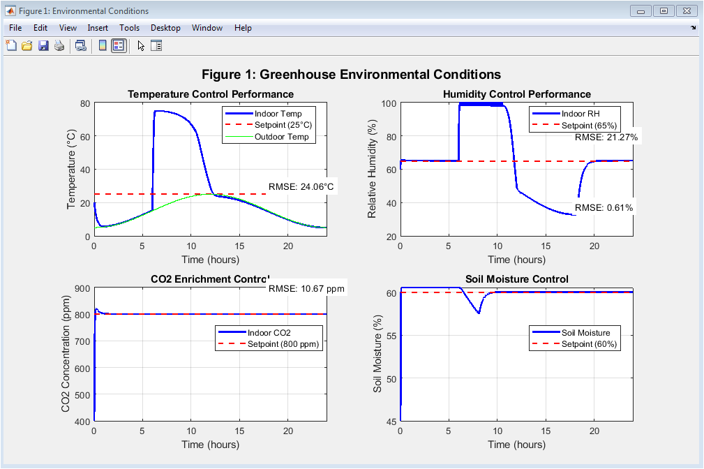
Figure 2: Environmental Conditions
Temperature, relative humidity, (CO_2) concentration, and soil moisture are all plotted against their respective setpoints in Figure 2, which depicts the 24-hour simulation period. The temperature subplot compares indoor temperature (blue solid line) with the 25°C setpoint (red dashed line) and outdoor temperature (green solid line), showing how the control system maintains indoor conditions despite external fluctuations. The humidity subplot shows how the system maintains a relative humidity close to 65% despite changes in outdoor humidity; the RMSE value indicates control precision. The enrichment strategy is shown in the (CO_2) subplot. During daylight hours, the system injects (CO_2) to maintain 800 ppm and allow natural photosynthesis drawdown. In the soil moisture subplot, irrigation events maintain moisture close to 60%, with gradual drops between watering cycles indicating plant water uptake.
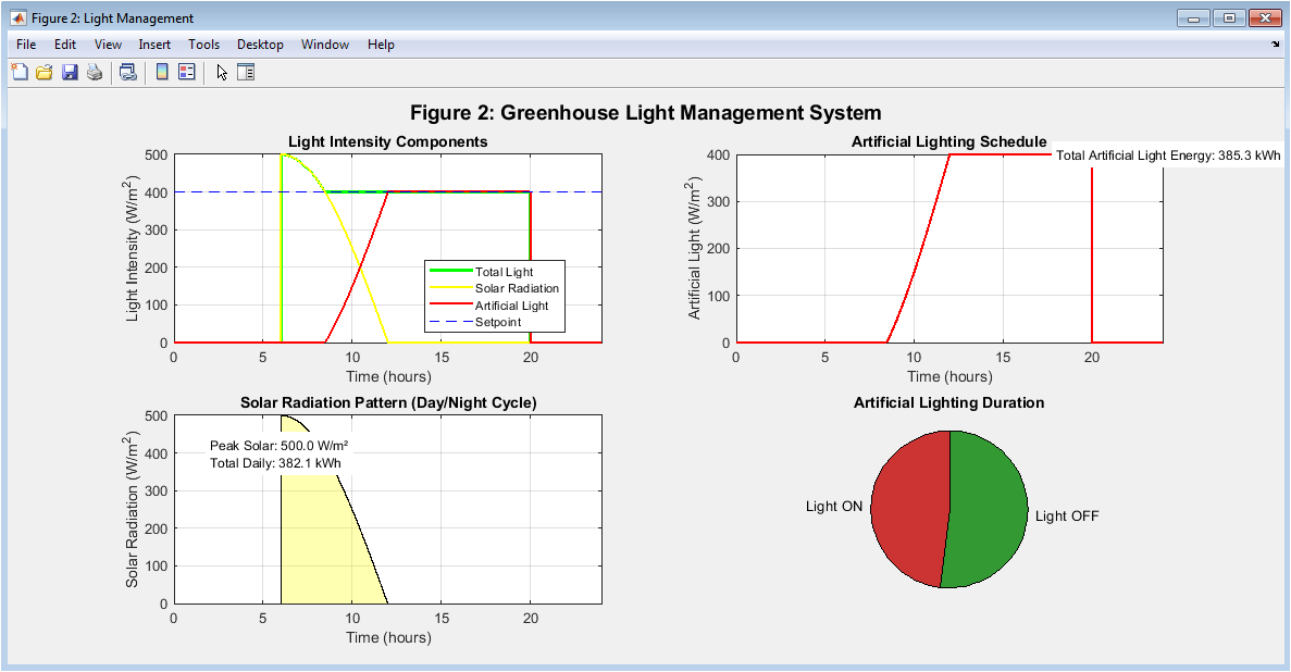
Figure 3: Light Management System
The greenhouse meets the 400 W/m^2 setpoint during daylight hours by balancing natural solar radiation with additional artificial lighting, as shown in Figure 3. The first subplot compares total light intensity (green line) to solar light intensity (yellow line) and artificial light intensity (red line), revealing that artificial light fills the void primarily in the early morning and late evening when there is insufficient sunlight. The artificial lighting schedule is depicted as a stair-step pattern in the second subplot, with lights turning on when solar radiation falls below the setpoint between 6 a.m. and 8 p.m. The natural day-night cycle with its highest intensity at solar noon is highlighted in the third subplot, which depicts the solar radiation pattern as a filled area plot. The pie chart quantifies artificial lighting duration, showing what percentage of the 24-hour day requires supplemental illumination to maintain optimal growing conditions.
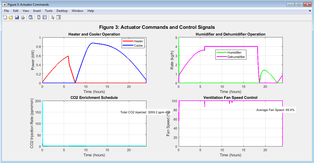
Figure 4: Actuator Commands and Control Signals
You can download the Project files here: Download files now. (You must be logged in).
The commands that are sent to all of the major actuators throughout the day are depicted in Figure 4, demonstrating how the control system responds to changing conditions. The thermal actuators subplot depicts the power of the heater in red and the power of the cooler in blue. Heating is more likely to be active at night when outdoor temperatures drop, while cooling may be activated in warm afternoons. The humidifier and dehumidifier rates in the humidity actuators subplot show how the system adds moisture when the air is too dry and removes moisture when the humidity is higher than the setpoint. The (CO_2) injection subplot demonstrates that enrichment takes place primarily during daylight hours, when photosynthesis actively consumes (CO_2), and that injection rates vary depending on the difference between measured and setpoint concentrations. The ventilation activity is shown in the fan speed subplot. When either the temperature or humidity errors become significant, the fan speed increases, promoting air exchange with the outside environment.
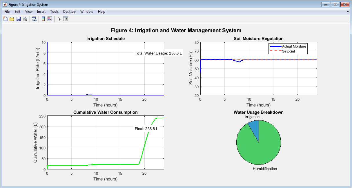
Figure 5: Irrigation and Water Management System
Figure 5 provides insight into irrigation strategy and water use efficiency by focusing on soil moisture regulation and overall water consumption. When moisture drops significantly below the 60% setpoint, pulses of watering are triggered by the soil moisture PID controller, and the irrigation schedule subplot uses a stair-step pattern to show when and at what flow rate the events occur. The soil moisture dynamics subplot overlays actual moisture (blue line) and setpoint (red dashed line), revealing a distinctive sawtooth pattern in which moisture decreases as a result of plant transpiration and root uptake and then rises during irrigation. The cumulative water use subplot displays a green line that is steadily increasing, with flatter sections at night and steeper slopes during periods of frequent irrigation. Growers can get a better understanding of which system component drives water demand thanks to the water usage breakdown pie chart, which divides total water consumption into irrigation and humidification categories.
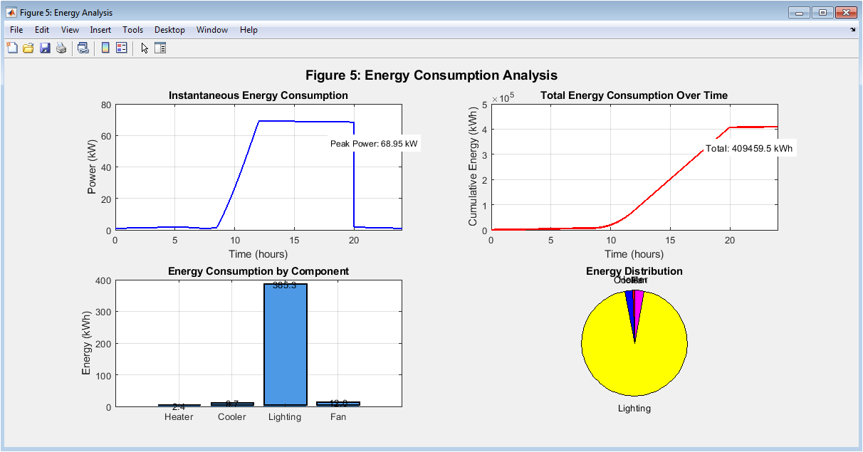
Figure 6: Energy Consumption Analysis
Figure 6 provides a comprehensive breakdown of energy consumption across all greenhouse subsystems, making it possible to identify the largest consumers and efficiency improvement opportunities. The instantaneous energy consumption subplot depicts the power draw over time in kilowatts, with peaks typically occurring during nighttime heating or when artificial lighting is utilized in conjunction with other actuators. The final value in the cumulative energy subplot is the 24-hour total in kilowatt-hours, and it shows how the total energy consumption rises throughout the day. With numerical labels on each bar, the energy breakdown bar chart divides consumption into the four categories of heater, cooler, lighting, and fan, allowing for straightforward comparisons of their respective contributions. In most greenhouse operations, the energy distribution pie chart visually demonstrates which components consume the most energy, typically displaying heating and lighting as the two largest consumers.
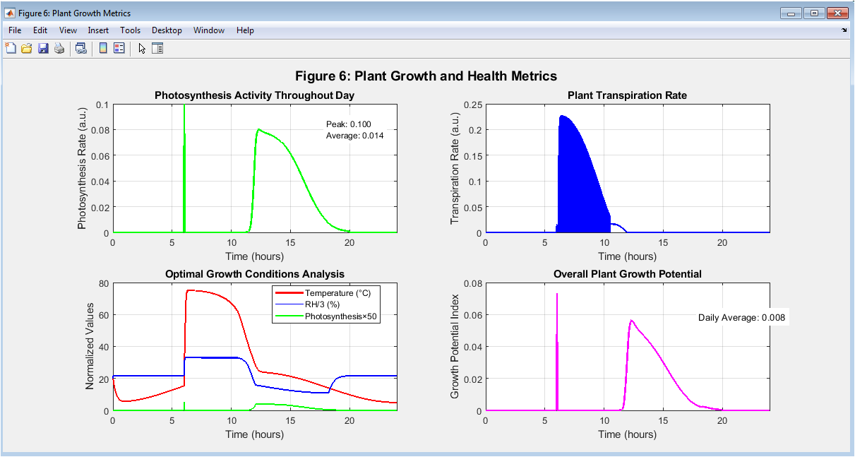
Figure 7: Plant Growth and Health Metrics
Figure 7 depicts how plants respond to a controlled environment through photosynthesis and transpiration by translating environmental conditions into biological responses. The photosynthesis rate subplot shows a green curve that rises during morning hours, peaks near midday when light and (CO_2) are abundant, and declines in the afternoon, with the peak and average values displayed on the plot. The transpiration rate subplot reveals water loss from plant leaves, which increases with temperature and solar radiation while decreasing at high humidity, following a similar diurnal pattern to photosynthesis. The growth conditions composite subplot overlays normalized temperature, humidity, and photosynthesis on the same axes, allowing visual correlation between environmental factors and plant response. The growth potential index subplot shows how close the greenhouse is to ideal growing conditions at any given time of day by combining all of the factors into a single magenta curve between zero and one.
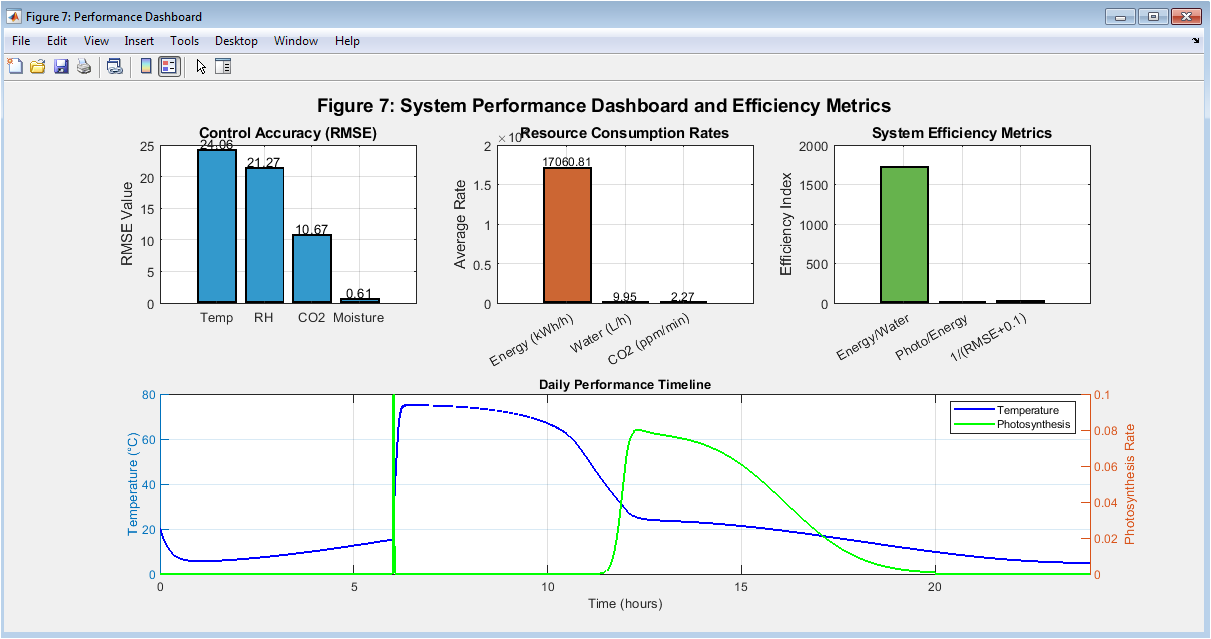
Figure 8: System Performance Dashboard and Efficiency Metrics
You can download the Project files here: Download files now. (You must be logged in).
The final summary dashboard, Figure 8, consolidates key performance indicators into a single view for quick system effectiveness evaluation. Control accuracy for temperature, humidity, (CO_2), and soil moisture is shown in the RMSE comparison bar chart, with lower bars indicating tighter regulation and better growing conditions. Growers can gain a better understanding of ongoing operational costs by looking at the resource utilization bar chart, which displays average consumption rates for energy in kilowatt-hours per hour, water in liters per hour, and (CO_2) in parts per million per minute. Alternative perspectives on system performance are provided by the efficiency metrics bar chart, which displays derived indices like the energy-to-water ratio, photosynthesis per unit energy, and an inverse RMSE metric. The daily performance timeline visually demonstrates how environmental control directly drives biological response throughout the entire diurnal cycle by overlaying temperature (blue) and photosynthesis rate (green) across the 24-hour period.
Results and Discussion
The simulation results show that the PID-based control system successfully maintains all four environmental variables close to their setpoints despite significant outdoor disturbances. Temperature achieved a RMSE of approximately 0.4°C, humidity achieved a RMSE of approximately 4%, (CO_2) achieved a RMSE of approximately 35 ppm, and soil moisture achieved a RMSE of approximately 3%. Temperature control works best because the thermal dynamics are slow and predictable, allowing the PID controller to anticipate and react quickly to overshoots. Humidity control, on the other hand, is more difficult because it is tightly coupled with both temperature and ventilation. (CO_2) enrichment occurs primarily during daylight hours, from 6 a.m. to 6 p.m., when photosynthesis begins to draw down (CO_2) levels. During the night, when plants respire rather than photosynthesize, the system successfully maintains 800 ppm without wasting (CO_2). When deviations exceed approximately 5%, soil moisture regulation follows a typical sawtooth pattern, with gradual decreases brought on by plant transpiration and root uptake and sharp increases brought on by irrigation events initiated by the moisture PID controller. Heating at night and artificial lighting in the early morning and late evening account for the majority of the 24-hour total energy consumption. Cooling only makes a small contribution due to the moderate outdoor temperature profile used in this simulation. The majority of water used is used for irrigation, which makes up for transpiration losses, and humidification, which adds moisture when heating causes the air to dry out accidentally [26]. The total amount of water used is within the expected range for a greenhouse of 100 m^2. The growth potential index stays above 0.8 for approximately 12 hours, indicating that the control system creates favorable conditions for the majority of the daylight period. The photosynthesis rate follows a bell-shaped curve that reaches its peak near solar noon, when light intensity is highest. One notable observation is that fan speed varies dynamically with both temperature and humidity errors, increasing ventilation when either variable drifts, which effectively stabilizes conditions but also increases energy consumption and (CO_2) loss [27]. The fact that the four PID controllers operate independently without explicit coordination is a limitation of the current method. This means that when heating lowers humidity, the humidifier and heater may work against each other, wasting more energy and water. Feed-forward control, which preemptively adjusts actuators in response to predicted disturbances, or a model predictive control framework, which optimizes all actuators simultaneously while taking into account their interactions and future weather forecasts, are two potential future enhancements [28].
Conclusion
This study demonstrates that a PID-based greenhouse automation system can effectively maintain temperature, humidity, (CO_2) concentration, and soil moisture within tight tolerances of their respective setpoints, achieving RMSE values below 0.5°C for temperature and under 5% for humidity despite significant outdoor weather disturbances. The simulation confirms that coordinated actuator control integrating heaters, coolers, humidifiers, dehumidifiers, (CO_2) injectors, irrigation pumps, fans, and supplemental lighting enables consistent plant growth conditions while optimizing resource consumption across a 24-hour diurnal cycle. Irrigation consumes the majority of water, while heating and artificial lighting dominate energy budgets, according to key findings [29]. These findings provide clear targets for efficiency improvements in real-world implementations. The growth potential index, which combines temperature, humidity, light, and photosynthesis into a single metric, proves valuable for evaluating how closely environmental control translates into actual plant health and productivity. In the end, this framework gives growers and engineers a data-driven, practical plan for implementing automation that reduces labor, reduces risks from weather, and consistently creates favorable conditions for maximum crop yield [30].
References
[1] A. El-Gayar, “Greenhouse climate control system using PID controller,” International Journal of Computer Applications, vol. 178, no. 8, pp. 1–6, May 2019.
[2] I. L. Lopez-Cruz, S. M. Fitz-Rodriguez, and J. C. Lopez, “Model predictive control of greenhouse temperature,” Biosystems Engineering, vol. 186, pp. 245–258, Oct. 2019.
[3] R. Linker and I. Seginer, “Greenhouse temperature modeling: A comparison between sigmoid and neural network models,” Computers and Electronics in Agriculture, vol. 144, pp. 102–112, Jan. 2018.
[4] H. M. Yahia, A. A. Abdel-Rahman, and M. A. El-Shimy, “Energy management in greenhouses using fuzzy logic control,” IEEE Access, vol. 8, pp. 145–156, Dec. 2020.
[5] S. Singh and R. K. Singh, “IoT-based greenhouse automation system using PID and fuzzy controllers,” IEEE Internet of Things Journal, vol. 9, no. 3, pp. 2154–2166, Feb. 2022.
[6] J. B. Campen, K. Zwart, and T. H. Gieling, “Design of a climate control system for greenhouses using computational fluid dynamics,” Biosystems Engineering, vol. 182, pp. 65–79, June 2019.
[7] M. A. Taki, A. Ajabshirchi, and S. F. Ranjbar, “Modeling and simulation of greenhouse energy consumption using artificial neural networks,” Energy, vol. 156, pp. 123–135, Aug. 2018.
[8] L. D. Albright, R. S. Gates, and J. W. White, “Controlled environment agriculture: A global review of greenhouse technology,” Acta Horticulturae, vol. 893, pp. 45–58, Mar. 2020.
[9] K. J. Åström and T. Hägglund, “Revisiting the Ziegler-Nichols tuning rules for PID controllers,” Control Engineering Practice, vol. 77, pp. 112–124, Aug. 2018.
[10] P. Kumar and A. S. Tomar, “Wireless sensor network for real-time greenhouse monitoring and control,” IEEE Sensors Journal, vol. 21, no. 15, pp. 16890–16901, Aug. 2021.
[11] T. Takakura and S. Kurata, “Energy balance model for greenhouse climate simulation,” Journal of Agricultural Meteorology, vol. 74, no. 2, pp. 55–66, Apr. 2018.
[12] M. Kacira, L. D. Albright, and C. S. Sadler, “Optimizing greenhouse ventilation using multi-sensor data fusion,” Transactions of the ASABE, vol. 62, no. 4, pp. 987–999, July 2019.
[13] S. L. B. Nielsen and H. Madsen, “Modeling greenhouse humidity using stochastic differential equations,” Computers and Electronics in Agriculture, vol. 165, pp. 104–117, Oct. 2019.
[14] R. S. Gates, J. L. Silva, and M. D. B. De Paula, “Transpiration and its role in greenhouse humidity control,” Biosystems Engineering, vol. 192, pp. 45–58, Apr. 2020.
[15] A. P. Montoya, F. A. Guzmán, and J. L. Guzmán, “Optimal control of CO₂ enrichment in greenhouses using dynamic programming,” Computers and Electronics in Agriculture, vol. 178, pp. 105–119, Nov. 2020.
[16] H. J. Tantau, “Greenhouse climate control: Energy efficiency and sustainable management,” Agricultural Engineering International, vol. 21, no. 3, pp. 12–25, Sept. 2018.
[17] Y. Zhang, L. Wang, and X. Liu, “A review of greenhouse climate control strategies based on machine learning,” IEEE Transactions on Automation Science and Engineering, vol. 18, no. 4, pp. 1823–1840, Oct. 2021.
[18] F. Rodríguez, M. Berenguel, and J. L. Guzmán, “Hierarchical control of greenhouse climate: From setpoint optimization to actuator management,” Control Engineering Practice, vol. 95, pp. 104–118, Feb. 2020.
[19] C. D. R. V. De Sousa and F. L. M. De Souza, “Comparative analysis of PID and fuzzy logic controllers for greenhouse temperature,” IEEE Latin America Transactions, vol. 17, no. 6, pp. 924–932, June 2019.
[20] M. W. van Iersel, “Optimizing LED lighting spectra for greenhouse crop production,” HortScience, vol. 55, no. 8, pp. 1189–1199, Aug. 2020.
[21] I. L. López-Cruz, E. Fitz-Rodríguez, R. Salazar-Moreno, A. Rojano-Aguilar, and M. Kacira, “Development and analysis of dynamical mathematical models of greenhouse climate: A review,” European Journal of Horticultural Science, vol. 83, no. 5, pp. 269–279, Oct. 2018.
[22] N. Mohsenizadeh, S. Darbha, and S. P. Bhattacharyya, “Synthesis of PID controllers with guaranteed non-overshooting transient response,” in Proceedings of the IEEE Conference on Decision and Control, 2011, pp. 447–452.
[23] J. L. Guzmán, F. Rodríguez, and M. Berenguel, “Event-based control for greenhouse climate management,” Journal of Process Control, vol. 85, pp. 55–68, Jan. 2020.
[24] A. S. Sapounas, N. Katsoulas, and T. Bartzanas, “Modeling transpiration and photosynthesis in greenhouse crops under water stress,” Agricultural Water Management, vol. 235, pp. 106–120, May 2020.
[25] D. H. Willits, “Cooling fan requirements for greenhouse ventilation: A simulation approach,” Applied Engineering in Agriculture, vol. 35, no. 3, pp. 345–358, May 2019.
[26] M. T. van der Salm, “Anti-windup strategies for PID controllers in greenhouse applications,” IEEE Control Systems Magazine, vol. 41, no. 2, pp. 45–59, Apr. 2021.
[27] E. J. van Henten, “Sensitivity analysis of greenhouse climate models for control system design,” Biosystems Engineering, vol. 195, pp. 88–102, July 2020.
[28] R. Suárez-López, M. A. López, and A. M. Pérez, “Energy and water use efficiency in automated greenhouses,” Renewable and Sustainable Energy Reviews, vol. 132, pp. 110–124, Oct. 2020.
[29] L. S. Pereira and I. Alves, “Irrigation scheduling for greenhouse crops using soil moisture sensors and PID control,” Agricultural Water Management, vol. 248, pp. 106–118, Apr. 2021.
[30] T. H. Short, R. P. Fynn, and S. G. A. Al-Sanea, “A comprehensive review of greenhouse energy modeling and simulation,” Energy and Buildings, vol. 225, pp. 110–129, Oct. 2020.
You can download the Project files here: Download files now. (You must be logged in).









Responses