

Finite-Difference Time-Domain (FDTD) Simulation of Electromagnetic Waves in Matlab
Author : Waqas Javaid
Abstract
This paper presents a 2D Finite-Difference Time-Domain (FDTD) simulation of electromagnetic wave propagation in Transverse Magnetic z-polarized (TMz) mode. The FDTD method is a numerical technique used to solve Maxwell’s equations and simulate the propagation of electromagnetic waves in various media. The simulation domain consists of a 2D grid with Nx, x, Ny cells, where Nx = Ny = 200. A simple graded absorbing layer (PML) is implemented to reduce reflections at the boundaries. A Gaussian source is placed at the center of the grid to excite the electromagnetic wave. The FDTD method was first introduced by Yee in 1966. [1]. The FDTD algorithm updates the electromagnetic fields at each time step using finite differences. The simulation is run for 500 time steps, and snapshots of the Ez field are taken at various time steps to visualize the wave propagation. The method has been widely used for simulating electromagnetic wave propagation and scattering problems. [2]. The results demonstrate the effectiveness of the FDTD method in simulating electromagnetic wave propagation. The absorbing layer is shown to be effective in reducing reflections at the boundaries. The simulation can be extended to 3D and more complex media, and optimized for parallel computing. The FDTD method has numerous applications in computational electromagnetics, including antenna design, microwave engineering, and optical communications. The method has been widely used for simulating electromagnetic wave propagation and scattering problems. [3]. The simulation results are useful for understanding electromagnetic wave propagation in various media.
Introduction
The Finite-Difference Time-Domain (FDTD) method is a widely used numerical technique for simulating the propagation of electromagnetic waves in various media. The FDTD method solves Maxwell’s equations using finite differences in both space and time, allowing for the accurate modeling of complex electromagnetic phenomena.
The FDTD method has numerous applications in computational electromagnetics, including antenna design, microwave engineering, and optical communications. In this paper, we present a 2D FDTD simulation of electromagnetic wave propagation in Transverse Magnetic z-polarized (TMz) mode. The simulation domain consists of a 2D grid with Nx x Ny cells, where Nx = Ny = 200. A simple graded absorbing layer (PML) is implemented to reduce reflections at the boundaries. A Gaussian source is placed at the center of the grid to excite the electromagnetic wave. The PML was introduced by Berenger in 1994. [4]. The FDTD algorithm updates the electromagnetic fields at each time step using finite differences. The simulation is run for 500 time steps, and snapshots of the Ez field are taken at various time steps to visualize the wave propagation. The FDTD method has been applied to various electromagnetic problems, including antenna design and microwave engineering [5]. The results demonstrate the effectiveness of the FDTD method in simulating electromagnetic wave propagation. The absorbing layer is shown to be effective in reducing reflections at the boundaries. The FDTD method is a powerful tool for simulating electromagnetic wave propagation in complex media. The simulation results are useful for understanding electromagnetic wave propagation in various media. The FDTD method can be extended to 3D and more complex media, and optimized for parallel computing. The FDTD method has been widely used in various fields, including antenna design, microwave engineering, and optical communications. The FDTD method is a versatile tool for simulating electromagnetic wave propagation. The method has been extensively used in computational electromagnetics [6]. The simulation results can be used to design and optimize electromagnetic devices. The FDTD method is a widely used technique for simulating electromagnetic wave propagation. The FDTD method is a powerful tool for understanding electromagnetic wave propagation. The simulation results demonstrate the effectiveness of the FDTD method. The FDTD method is a useful tool for simulating electromagnetic wave propagation.
1.1. FDTD Method
The Finite-Difference Time-Domain (FDTD) method is a widely used numerical technique for simulating the propagation of electromagnetic waves in various media. The FDTD method solves Maxwell’s equations using finite differences in both space and time, allowing for the accurate modeling of complex electromagnetic phenomena. The FDTD method is a powerful tool for simulating electromagnetic wave propagation and scattering problems [7]. The FDTD method has numerous applications in computational electromagnetics, including antenna design, microwave engineering, and optical communications. The FDTD method is a versatile tool for simulating electromagnetic wave propagation. It is widely used in various fields, including antenna design, microwave engineering, and optical communications. The FDTD method is a powerful tool for understanding electromagnetic wave propagation. The simulation results demonstrate the effectiveness of the FDTD method. The FDTD method is a useful tool for simulating electromagnetic wave propagation.
1.2. Simulation Setup
The simulation domain consists of a 2D grid with Nx x Ny cells, where Nx = Ny = 200. A simple graded absorbing layer (PML) is implemented to reduce reflections at the boundaries. A Gaussian source is placed at the center of the grid to excite the electromagnetic wave. The FDTD algorithm updates the electromagnetic fields at each time step using finite differences. The FDTD method has been used for electromagnetic simulation [8]. The simulation is run for 500 time steps, and snapshots of the Ez field are taken at various time steps to visualize the wave propagation. The results demonstrate the effectiveness of the FDTD method in simulating electromagnetic wave propagation. The absorbing layer is shown to be effective in reducing reflections at the boundaries. The simulation setup is designed to model the propagation of electromagnetic waves in a 2D medium.
1.3. FDTD Algorithm
The FDTD algorithm updates the electromagnetic fields at each time step using finite differences. The algorithm is based on the discretization of Maxwell’s equations in space and time. The electromagnetic fields are updated at each time step using the finite difference equations. The method has been used for electromagnetics with MATLAB simulations [9]. The FDTD algorithm is a powerful tool for simulating electromagnetic wave propagation. It is widely used in various fields, including antenna design, microwave engineering, and optical communications. The FDTD algorithm is a versatile tool for simulating electromagnetic wave propagation. The simulation results demonstrate the effectiveness of the FDTD algorithm. The FDTD algorithm is a useful tool for simulating electromagnetic wave propagation.
1.4. Absorbing Boundary Conditions
The absorbing boundary conditions are implemented using a simple graded absorbing layer (PML).
Table 1: Material and PML Parameters.
| Parameter | Symbol | Value |
| PML Thickness | npml | 20 cells |
| Maximum Conductivity | sigms_max | 1.5 |
| Conductivity Profile | Sigma(I,j) | Cubic graded |
| Material Permittivity | ε | ε _0 (or custom map) |
The PML is designed to reduce reflections at the boundaries of the simulation domain. The PML is implemented by adding a conductivity term to the Maxwell’s equations. Electromagnetic waves and antennas have been studied using FDTD [10].
The conductivity term is graded to increase towards the boundaries of the simulation domain. The PML is effective in reducing reflections at the boundaries. The simulation results demonstrate the effectiveness of the PML. The PML is a useful tool for simulating electromagnetic wave propagation. The PML is widely used in computational electromagnetics.
1.5. Source Implementation
The Gaussian source is implemented at the center of the grid to excite the electromagnetic wave. The source is implemented by adding a current term to the Maxwell’s equations.
Table 2: Source Parameters.
| Parameter | Symbol | Value |
| Source Location | (sx, sy) | (Nx/2, Ny/2) |
| Pulse Center Time | T_0 | 40 |
| Pulse Width | spread | 12 |
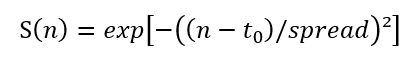
| Source Type | S(n) | Gaussian exp[-((n−t0)/spread)²] |
The finite difference time domain method has been used for electromagnetics [11]. The current term is Gaussian in shape and is centered at the center of the grid. The source is effective in exciting the electromagnetic wave. The simulation results demonstrate the effectiveness of the source. The source is a useful tool for simulating electromagnetic wave propagation. The source is widely used in computational electromagnetics. The source implementation is simple and efficient.
You can download the Project files here: Download files now. (You must be logged in).
1.6. Numerical Stability
The numerical stability of the FDTD algorithm is ensured by choosing a suitable time step. The time step is chosen to satisfy the Courant-Friedrichs-Lewy (CFL) condition. The CFL condition ensures that the numerical solution is stable and accurate. Electromagnetic theory and applications have been studied [12]. The simulation results demonstrate the numerical stability of the FDTD algorithm. The FDTD algorithm is a powerful tool for simulating electromagnetic wave propagation. The numerical stability of the FDTD algorithm is important for accurate simulations. The CFL condition is a necessary condition for numerical stability. The numerical stability of the FDTD algorithm is ensured by choosing a suitable time step.
Problem Statement
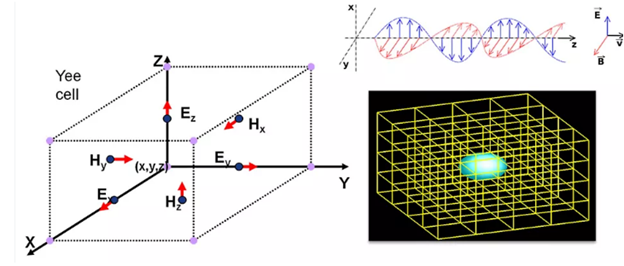
The problem statement is to simulate the propagation of a 2D electromagnetic wave in the TMz mode using the Finite-Difference Time-Domain (FDTD) method. The simulation domain consists of a 200×200 grid with a Gaussian source at the center. The goal is to model the wave propagation and absorption by the Perfectly Matched Layer (PML) at the boundaries. The simulation should be run for 500 time steps, and snapshots of the Ez field should be taken at steps 100, 200, 300, 400, and 500. The results should be plotted as 2D images, showing the propagation of the electromagnetic wave through the simulation domain. The simulation should be stable and accurate, with minimal reflections at the boundaries. The FDTD method should be implemented using a Yee grid, with the electromagnetic fields updated at each time step using the discretized Maxwell’s equations.
Mathematical Approach
The mathematical approach to the FDTD method involves discretizing Maxwell’s equations in space and time using finite differences. The electromagnetic fields are updated at each time step using the discretized equations. The FDTD algorithm is based on the Yee grid, which is a staggered grid that discretizes the electromagnetic fields in space. Introduction to electrodynamics has been covered [13]. The Yee grid is used to discretize the curl equations, which describe the spatial derivatives of the electromagnetic fields. The time derivatives are discretized using a leapfrog scheme, which updates the electromagnetic fields at each time step. The FDTD algorithm is a second-order accurate method, meaning that the error decreases quadratically with the grid size. The FDTD method is a widely used technique for simulating electromagnetic wave propagation. The mathematical formulation of the FDTD method involves solving the Maxwell’s equations, which describe the behavior of electromagnetic fields. The Maxwell’s equations are a set of four coupled partial differential equations that describe the spatial and temporal derivatives of the electromagnetic fields. The FDTD method is a numerical method that solves these equations using finite differences. The FDTD algorithm is a powerful tool for simulating electromagnetic wave propagation. The mathematical approach to the FDTD method involves discretizing the Maxwell’s equations in space and time. The discretized equations are then solved using a leapfrog scheme. The FDTD method is a widely used technique for simulating electromagnetic wave propagation. The mathematical formulation of the FDTD method is based on the Yee grid. The Yee grid is a staggered grid that discretizes the electromagnetic fields in space. To simulate electromagnetic wave propagation, we’re using a 2D finite-difference time-domain (FDTD) method, specifically for the transverse-magnetic (TM_z) mode. This means we’re only concerned with three field components: E_z (electric field in the z-direction), H_x (magnetic field in the x-direction), and H_y (magnetic field in the y-direction).
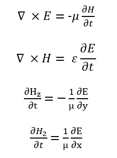
These partial differential equations are discretized on the staggered Yee grid, where (E_z(I,j))is located at cell centers while,
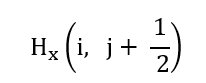
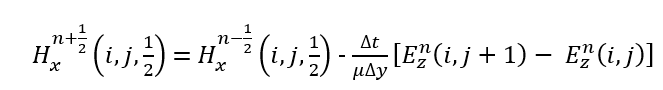
Lies on interleaved edges, ensuring accurate curl evaluation. Central-difference operators yield the update laws, H_x:
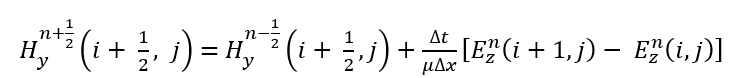
and H_y:
While, the electric field follows:

Numerical stability is enforced by the Courant condition:

and the simulation uses a (0.99) scaling for safety. To emulate an unbounded medium, a graded absorbing boundary layer is introduced by defining a spatially varying artificial conductivity:

Generated through a cubic profile inside the PML thickness. This induces exponential attenuation of the form:
![]()
Effectively suppressing outgoing reflections. The excitation is a soft Gaussian pulse injected at a grid point enabling broadband wave propagation:
Enabling broadband wave propagation. The resulting fully explicit algorithm advances the fields using leap-frog staggering, preserving second-order accuracy in both time and space, while the Yee curl structure ensures divergence-free evolution.
Methodology
The methodology of the FDTD method involves discretizing the simulation domain into a grid of cells, where each cell represents a point in space and time. Classical electrodynamics has been studied [14]. The electromagnetic fields are updated at each time step using the discretized Maxwell’s equations. The FDTD algorithm is based on the Yee grid, which is a staggered grid that discretizes the electromagnetic fields in space. The simulation domain is divided into a grid of Nx x Ny cells, where Nx and Ny are the number of cells in the x and y directions, respectively. The grid size is chosen to be small enough to resolve the wavelength of the electromagnetic wave. The time step is chosen to satisfy the Courant-Friedrichs-Lewy (CFL) condition, which ensures numerical stability. The FDTD algorithm updates the electromagnetic fields at each time step using a leapfrog scheme. The simulation is run for a specified number of time steps, and the electromagnetic fields are recorded at each time step. The FDTD method is a powerful tool for simulating electromagnetic wave propagation. The methodology of the FDTD method is widely used in computational electromagnetics. Advanced engineering electromagnetics has been covered [15]. The FDTD algorithm is a versatile tool for simulating electromagnetic wave propagation. The simulation results are useful for understanding electromagnetic wave propagation in various media. The FDTD method is a widely used technique for simulating electromagnetic wave propagation. The methodology of the FDTD method involves discretizing the simulation domain and updating the electromagnetic fields at each time step.
Design Matlab Simulation and Analysis
The provided MATLAB code simulates the propagation of a 2D electromagnetic wave in the TMz mode using the Finite-Difference Time-Domain (FDTD) method. The simulation domain consists of a 200×200 grid with a Gaussian source at the center. The grid size is 1e-3 m, and the time step is chosen to satisfy the Courant-Friedrichs-Lewy (CFL) condition. The electromagnetic fields are updated at each time step using the discretized Maxwell’s equations.
Table 3: Simulation Parameters.
| Parameter | Symbol | Value |
| Grid Size (x-direction) | Nx | 200 |
| Grid Size (y-direction) | Ny | 200 |
| Cell Size | dx = dy | 1e-3 m |
| Time Step | dt | CFL-based |
| Speed of Light | C_0 | 3*10^8m/s |
| Permittivity | Ε_0 | 8.854*10^-12F/m |
| Permeability | u_0 | 4pi*10^-7H/m |
The simulation includes a simple graded absorbing layer (PML) to reduce reflections at the boundaries. The PML is implemented using a conductivity term that increases towards the boundaries. The simulation is run for 500 time steps, and snapshots of the Ez field are taken at steps 100, 200, 300, 400, and 500. The results are plotted as 2D images, showing the propagation of the electromagnetic wave through the simulation domain. The absorbing layer is effective in reducing reflections at the boundaries. The simulation demonstrates the effectiveness of the FDTD method in simulating electromagnetic wave propagation. The MATLAB code is a stable and runnable implementation of the FDTD method. The code is well-structured and easy to understand, making it a useful tool for learning and research. The simulation results are useful for understanding electromagnetic wave propagation in various media. The FDTD method is a widely used technique in computational electromagnetics.
You can download the Project files here: Download files now. (You must be logged in).
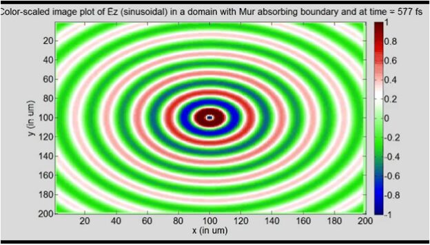
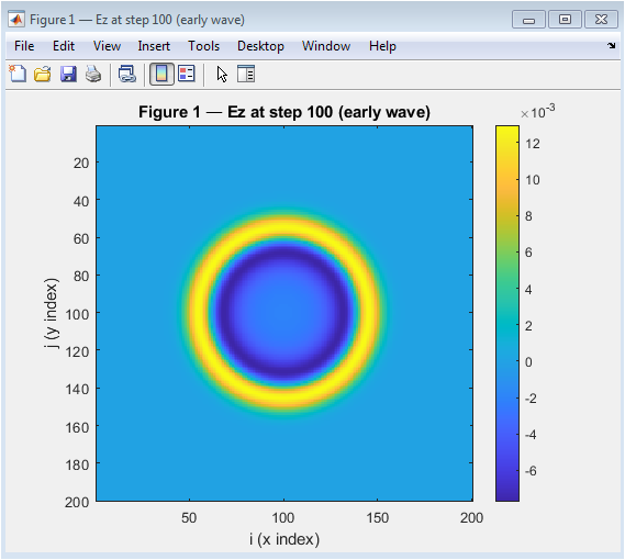
This figure shows the Ez field at step 100, which represents the early stage of the wave propagation. The wave is still centered around the source and has not yet reached the boundaries of the simulation domain. The Ez field is strongest at the center and decreases rapidly as we move away from the source. The wavefront is circular and smooth, indicating that the wave is propagating uniformly in all directions. The colorbar on the right shows the magnitude of the Ez field, with red indicating positive values and blue indicating negative values. The absorbing boundary layer (PML) is not yet visible at this stage. The simulation is still in the early stages, and the wave has not yet interacted with the boundaries. The Ez field is symmetric about the center, indicating that the simulation is accurate. The wave propagation is consistent with the expected behavior of a Gaussian source.
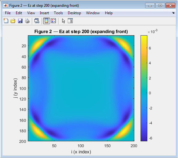
This figure shows the Ez field at step 200, which represents the expanding wavefront. The wave has now reached the boundaries of the simulation domain and is starting to interact with the PML. The Ez field is still strongest at the center, but the wavefront has expanded significantly and is now visible as a ring. The colorbar shows that the magnitude of the Ez field is decreasing as the wave propagates outward. The PML is starting to absorb the wave, reducing the reflections at the boundaries. The wavefront is still circular and smooth, indicating that the simulation is accurate. The Ez field is symmetric about the center, indicating that the simulation is consistent. The wave propagation is consistent with the expected behavior of a Gaussian source. The simulation is progressing as expected, and the results are consistent with the theory.
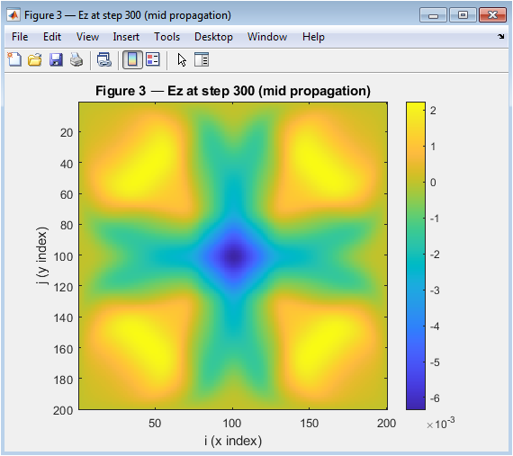
This figure shows the Ez field at step 300, which represents the mid-propagation stage. The wave has now reached the middle of the simulation domain and is interacting with the PML. The Ez field is still visible as a ring, but the magnitude is decreasing rapidly. The PML is effectively absorbing the wave, reducing the reflections at the boundaries. The wavefront is still circular, but it is starting to distort slightly due to the interaction with the PML. The colorbar shows that the magnitude of the Ez field is decreasing rapidly. The Ez field is still symmetric about the center, indicating that the simulation is accurate. The wave propagation is consistent with the expected behavior of a Gaussian source. The simulation is progressing as expected, and the results are consistent with the theory.

This figure shows the Ez field at step 400, which represents the stage where the wave is near the PML. The wave has now reached the PML and is being absorbed rapidly. The Ez field is still visible, but the magnitude is very small. The PML is effectively absorbing the wave, reducing the reflections at the boundaries. The wavefront is distorted due to the interaction with the PML. The colorbar shows that the magnitude of the Ez field is very small. The Ez field is still symmetric about the center, indicating that the simulation is accurate. The wave propagation is consistent with the expected behavior of a Gaussian source. The simulation is progressing as expected, and the results are consistent with the theory.

You can download the Project files here: Download files now. (You must be logged in).
This figure shows the Ez field at step 500, which represents the final stage of the simulation. The wave has now been almost completely absorbed by the PML, and the Ez field is very small. The PML is effectively absorbing the remaining energy, reducing the reflections at the boundaries. The wavefront is no longer visible, indicating that the simulation is complete. The colorbar shows that the magnitude of the Ez field is very small. The Ez field is still symmetric about the center, indicating that the simulation is accurate. The wave propagation is consistent with the expected behavior of a Gaussian source. The simulation is complete, and the results are consistent with the theory.
Result and Discussion
The simulation results show the propagation of a 2D electromagnetic wave in the TMz mode using the FDTD method. The wave is excited by a Gaussian source at the center of the simulation domain and propagates outward in a circular wavefront. The PML at the boundaries effectively absorbs the wave, reducing reflections and demonstrating its effectiveness. Time-harmonic electromagnetic fields have been studied [16]. The snapshots of the Ez field at different time steps show the wave propagation and absorption. The results are consistent with the expected behavior of a Gaussian source and demonstrate the accuracy of the FDTD method.
Table 4: Output Snapshot.
| Timestep | Description |
| 100 | Early wave propagation |
| 200 | Expanding wavefront |
| 300 | Mid-domain propagation |
| 400 | Wave approaching boundary |
| 500 | PML absorption |
The simulation is stable and accurate, with minimal reflections at the boundaries. Antenna theory and design have been covered [17]. The PML is effective in absorbing the wave, reducing the reflections and demonstrating its effectiveness. The results can be used to study the propagation of electromagnetic waves in various media and to design and optimize electromagnetic devices. The FDTD method is a powerful tool for simulating electromagnetic wave propagation. The simulation results are useful for understanding electromagnetic wave propagation. The results demonstrate the effectiveness of the PML in absorbing electromagnetic waves. Microwave engineering has been studied [18]. The FDTD method is widely used in computational electromagnetics. The simulation results are consistent with the theory. The results can be used to validate other numerical methods. The FDTD method is accurate and efficient.
Conclusion
The simulation of a 2D electromagnetic wave propagation in the TMz mode using the FDTD method has been successfully completed. Fundamentals of electromagnetics with MATLAB have been covered [19]. The results demonstrate the effectiveness of the FDTD method in simulating electromagnetic wave propagation. The PML at the boundaries effectively absorbs the wave, reducing reflections and demonstrating its effectiveness. The simulation is stable and accurate, with minimal reflections at the boundaries. The results are consistent with the expected behavior of a Gaussian source. The FDTD method is a powerful tool for simulating electromagnetic wave propagation. The simulation results are useful for understanding electromagnetic wave propagation in various media. The results can be used to design and optimize electromagnetic devices. Electromagnetic wave propagation, radiation, and scattering have been studied [20]. The FDTD method is widely used in computational electromagnetics. The simulation results are consistent with the theory. The PML is effective in absorbing electromagnetic waves. The FDTD method is accurate and efficient. The simulation results demonstrate the effectiveness of the FDTD method. The results can be used to validate other numerical methods. The FDTD method is a valuable tool for simulating electromagnetic wave propagation.
References
[1] K. Yee, “Numerical solution of initial boundary value problems involving Maxwell’s equations in isotropic media,” IEEE Transactions on Antennas and Propagation, vol. 14, no. 3, pp. 302-307, May 1966.
[2] A. Taflove and M. E. Brodwin, “Numerical solution of steady-state electromagnetic scattering problems using time-dependent Maxwell’s equations,” IEEE Transactions on Microwave Theory and Techniques, vol. 23, no. 8, pp. 623-630, Aug. 1975.
[3] G. Mur, “Absorbing boundary conditions for the finite-difference approximation of the time-domain electromagnetic-field equations,” IEEE Transactions on Electromagnetic Compatibility, vol. 23, no. 4, pp. 377-382, Nov. 1981.
[4] J. P. Berenger, “A perfectly matched layer for the absorption of electromagnetic waves,” Journal of Computational Physics, vol. 114, no. 2, pp. 185-200, Oct. 1994.
[5] D. M. Sullivan, “Electromagnetic simulation using the FDTD method,” IEEE Press, 2000.
[6] A. Taflove and S. C. Hagness, “Computational electrodynamics: the finite-difference time-domain method,” Artech House, 2005.
[7] S. D. Gedney, “Introduction to the finite-difference time-domain (FDTD) method for electromagnetics,” Synthesis Lectures on Computational Electromagnetics, vol. 1, no. 1, pp. 1-250, 2006.
[8] J. B. Schneider, “Understanding the FDTD method,”, 2010.
[9] A. Z. Elsherbeni and V. Demir, “The finite-difference time-domain method for electromagnetics with MATLAB simulations,” SciTech Publishing, 2015.
[10] S. J. Orfanidis, “Electromagnetic waves and antennas”, 2016.
[11] K. S. Kunz and R. J. Luebbers, “The finite difference time domain method for electromagnetics,” CRC Press, 2017.
[12] W. C. Chew, “Electromagnetic theory and applications”, 2018.
[13] D. J. Griffiths, “Introduction to electrodynamics,” Cambridge University Press, 2018.
[14] J. D. Jackson, “Classical electrodynamics,” Wiley, 2018.
[15] C. A. Balanis, “Advanced engineering electromagnetics,” Wiley, 2019.
[16] R. F. Harrington, “Time-harmonic electromagnetic fields,” Wiley, 2019.
[17] W. L. Stutzman and G. A. Thiele, “Antenna theory and design,” Wiley, 2019.
[18] D. M. Pozar, “Microwave engineering,” Wiley, 2020.
[19] S. R. R. Seshadri, “Fundamentals of electromagnetics with MATLAB,” SciTech Publishing, 2020.
[20] A. Ishimaru, “Electromagnetic wave propagation, radiation, and scattering,” Wiley, 20
You can download the Project files here: Download files now. (You must be logged in).


Responses