

Matlab Simulation and Analysis of Extended Kalman Filter SLAM with Complete Diagnostic Metrics
Author : Waqas Javaid
Abstract
This paper presents a comprehensive implementation and analysis of an Extended Kalman Filter (EKF) for Simultaneous Localization and Mapping (SLAM). A high-fidelity MATLAB simulation is developed to model a mobile robot with range and bearing sensors navigating in an environment with unknown landmarks. The framework features a full prediction-update cycle with process and measurement noise, alongside a simple data association mechanism [1]. The robot’s pose uncertainty and landmark covariances are explicitly estimated and propagated through the system’s joint state. Performance is rigorously evaluated through extensive visualization, including trajectory comparisons, innovation sequences, and 2σ uncertainty ellipses. A key contribution is the formal consistency analysis using Normalized Estimation Error Squared (NEES), benchmarked against a χ² distribution. Results demonstrate the filter’s ability to concurrently estimate an accurate robot trajectory and a sparse feature map while quantifying estimation confidence [2]. The simulation provides a complete diagnostic suite for understanding EKF-SLAM characteristics, trade-offs, and failure modes, serving as a valuable tool for algorithm development and validation [3].
Introduction
Simultaneous Localization and Mapping (SLAM) stands as one of the fundamental challenges in autonomous robotics, enabling vehicles to operate in unknown environments without a priori maps [4].
The core objective is to enable a robot to incrementally build a consistent map of its surroundings while simultaneously estimating its own location within that map. Among early and foundational solutions, the Extended Kalman Filter (EKF) provides a probabilistic framework for tackling this joint estimation problem by maintaining a Gaussian representation of the state uncertainty. The EKF-SLAM algorithm elegantly formulates the problem by concatenating the robot’s pose and the positions of observed landmarks into a single state vector, whose full covariance matrix captures all cross-correlations. This approach, while computationally intensive for large-scale environments, offers a clear and mathematically rigorous method for understanding uncertainty propagation, data association, and filter consistency [5]. However, the performance of EKF-SLAM is highly sensitive to model linearizations, sensor noise characteristics, and the correctness of data associations between measurements and map features [6]. This necessitates thorough simulation-based analysis to characterize its behavior, validate its statistical consistency, and expose its limitations under realistic conditions [7]. The simulation incorporates key aspects such as landmark initialization, nearest-neighbor data association, and comprehensive diagnostic visualization. A primary contribution is the rigorous consistency analysis using the Normalized Estimation Error Squared (NEES) metric, testing whether the filter’s self-reported uncertainty accurately reflects the true estimation error [8]. By providing complete access to ground truth, our framework allows for an unambiguous evaluation of estimation errors, covariance growth, and overall system performance, serving as an essential educational and development tool for advanced robotics research [9].
1.1 The SLAM and its Foundational Role
The ability of a mobile robot to autonomously navigate and operate in a previously unknown environment is contingent upon solving the Simultaneous Localization and Mapping (SLAM) problem. This core challenge requires the robot to perform two interdependent tasks concurrently: constructing a model (map) of its surroundings and estimating its own position and orientation (pose) within that map. Without this capability, true autonomy in exploration, search and rescue, or planetary roving is impossible [10]. The problem is inherently probabilistic, as the robot must reason about its own motion, which is subject to control noise, and interpret sensor measurements, which are corrupted by observation noise, all while dealing with the inherent ambiguity of an unknown world. The solution is not merely a state estimate but a joint estimate of both the robot’s trajectory and the map, along with a full quantification of the uncertainty in this estimate. This paper focuses on one of the seminal, probabilistic approaches to this problem, the Extended Kalman Filter for SLAM, which provides a mathematically elegant, albeit linearized, solution framework for small- to medium-scale environments [11].
1.2 The EKF Framework for State Estimation in SLAM
The Extended Kalman Filter (EKF) serves as the estimation engine in the classic EKF-SLAM formulation. It extends the linear Kalman Filter to nonlinear systems by using local linearization (first-order Taylor expansion) of the motion and observation models around the current state estimate. In the context of SLAM, the state vector is uniquely composed, encapsulating not only the robot’s pose typically its x, y coordinates and heading but also the estimated coordinates of every landmark (e.g., distinct features) identified in the environment [12]. This creates a single, large, multi-dimensional state that evolves over time. The filter maintains a full covariance matrix for this state, which is crucial as it explicitly represents the uncertainty in the robot’s pose, the uncertainty in each landmark’s position, and, most importantly, the correlations (cross-covariances) between them. These correlations are key; they encode how information gained from observing a landmark reduces uncertainty not just for that landmark, but also for the robot’s own pose and all other correlated landmarks [13].
1.3 The Algorithm, Prediction, Association, and Update
The EKF-SLAM algorithm operates in a continuous cycle of three main phases. First, the Prediction Step uses the robot’s control inputs (e.g., velocity, steering angle) to propagate the estimated robot pose forward in time according to a motion model, while also updating the entire state covariance matrix to reflect the increased uncertainty from noisy actuation. Second, the robot obtains sensor measurements (e.g., range and bearing to perceived features). Before these can be used, the critical Data Association step must determine which, if any, of the observed features correspond to previously mapped landmarks [[14]. This work employs a simple nearest-neighbor method, matching new observations to existing map features based on statistical distance (Mahalanobis distance). Incorrect association is a primary cause of filter divergence. Finally, in the Update Step, the difference between the actual sensor measurements and the predicted measurements (the innovation) is used to correct the entire state vector and its covariance, tightening the estimates of both the robot and the observed landmarks.
1.4 The Imperative for Rigorous Simulation and Analysis
Theoretical understanding of EKF-SLAM must be complemented by practical implementation and empirical analysis to reveal its true characteristics and limitations. Real-world robot testing is expensive and often obscures underlying algorithmic behavior with hardware-specific noise and failures. Therefore, a high-fidelity, software-based simulation environment is an indispensable tool for development and validation. Such a simulation allows for complete control over all system parameters, including sensor noise characteristics, landmark distributions, and robot trajectories, while providing perfect access to ground truth data [15]. This enables unambiguous performance evaluation, allowing researchers to isolate algorithmic flaws from hardware issues. MATLAB simulation is designed for this exact purpose, implementing the complete EKF-SLAM pipeline with a configurable robot model, simulated landmarks, and realistic range-bearing sensors to create a controlled testbed for in-depth analysis [16].
1.5 System Models
Simulation implements detailed mathematical models for both robot kinematics and sensor characteristics.
Table 1: Noise Parameters
| Noise Type | Standard Deviation |
| Velocity Noise | 0.05 m/s |
| Angular Velocity Noise | 0.02 rad/s |
| Range Noise | 0.1 m |
| Bearing Noise | 0.05 rad |
| Landmark Initialization Noise | 0.1 m |
The robot follows a kinematic bicycle model, where control inputs consist of linear velocity and steering angle, with realistic Gaussian noise added to simulate actuator imperfections. The environment consists of randomly distributed static landmarks that serve as features for mapping. The robot is equipped with a simulated range-bearing sensor that provides polar coordinates (distance and angle) to visible landmarks within a defined field-of-view and maximum range. This sensor model incorporates realistic Gaussian noise in both range and bearing measurements, mimicking the limitations of real sensors like lidar or stereo cameras [17]. The complete simulation framework allows for systematic variation of all noise parameters, landmark density, and robot trajectories, enabling parametric studies of EKF-SLAM performance under different operating conditions.
1.6 Data Association Challenges and Solutions
One of the most critical aspects of SLAM implementation is the data association problem—correctly matching current sensor observations to existing map features or initializing new ones. Our implementation includes a probabilistic data association method based on the Mahalanobis distance between predicted and actual measurements. For each observation, we calculate the innovation covariance and determine statistical compatibility with existing landmarks. When no compatible landmark exists, a new landmark is initialized and added to the state vector with appropriate uncertainty [18]. The simulation also maintains an association table to track landmark correspondences throughout the mission. This mechanism allows us to study association failures and their catastrophic effects on filter consistency, as well as evaluate the robustness of the association logic under varying sensor noise levels and landmark densities.
1.7 Covariance Management and State Augmentation
As new landmarks are discovered, the EKF-SLAM state vector must be dynamically expanded through a process called state augmentation. Our implementation carefully handles this expansion by adding the new landmark’s estimated position to the state vector and appropriately expanding the covariance matrix. The initialization uncertainty for new landmarks is calculated based on the current robot pose uncertainty and the measurement noise characteristics [19]. The covariance matrix grows quadratically with the number of landmarks, which presents computational challenges for large-scale environments. Our simulation allows visualization of how these cross-covariances between robot pose and landmarks evolve over time, demonstrating how information from observing one landmark reduces uncertainty in other parts of the map through these correlation terms.
1.8 Performance Metrics and Diagnostic Tools
To comprehensively evaluate filter performance, we implement multiple diagnostic metrics beyond simple position error. These include: trajectory error statistics (mean, RMS, maximum), landmark estimation accuracy, innovation sequence analysis to verify whiteness properties, and NEES calculations for consistency checking [20]. The simulation generates extensive visualizations including 2σ uncertainty ellipses for both robot pose and landmark positions, covariance evolution plots, and error distribution histograms. These tools allow for thorough debugging and performance characterization. Particularly important is the innovation sequence analysis, which checks whether the innovations (difference between predicted and actual measurements) have zero mean and covariance matching the innovation covariance key indicators of a properly tuned filter [21].
1.9 Limitations and Practical Considerations
While EKF-SLAM provides a mathematically elegant solution, our simulation clearly reveals its practical limitations. The computational complexity grows quadratically with the number of landmarks, making it unsuitable for large-scale environments. Linearization errors accumulate during sharp turns or when uncertainty becomes large, potentially leading to filter divergence. The assumption of Gaussian noise distributions may not hold in real environments with outliers and multi-modal uncertainties [22]. Data association becomes increasingly challenging as the map grows, and incorrect associations can cause catastrophic filter failure. Our simulation allows users to explore these limitations by adjusting parameters to create challenging scenarios such as closing large loops or operating with highly noisy sensors demonstrating where the basic EKF-SLAM approach breaks down.
1.10 Educational Value and Research Applications
This simulation framework serves multiple purposes in robotics education and research. For students, it provides a hands-on tool to understand the complete SLAM pipeline from sensor measurements to final map, with full visibility into intermediate steps. For researchers, it offers a baseline implementation against which more advanced algorithms (FastSLAM, graph-based SLAM, or modern optimization-based approaches) can be compared. The modular design allows easy substitution of different motion models, sensor models, or data association algorithms [23]. By providing both the implementation and comprehensive analysis tools, this work bridges the gap between theoretical understanding and practical implementation, enabling deeper investigation into SLAM fundamentals and serving as a springboard for developing more robust solutions.
1.11 Future Extensions and Advanced Features
The current implementation provides a foundation that can be extended in several directions. Future work could incorporate more sophisticated data association methods like Joint Compatibility Branch and Bound (JCBB) to handle ambiguous environments [24]. The framework could be extended to include multiple robots (multi-agent SLAM) or different sensor modalities such as visual features. Implementation of submap techniques or switching to an information filter representation could address scalability issues. Additional features could include loop closure detection and handling, which is crucial for reducing accumulated drift over long trajectories. The simulation architecture also supports integration with real sensor data, providing a pathway from simulation to real-world deployment while maintaining the same analysis tools for performance evaluation across both domains.
Problem Statement
The central challenge addressed in this work is the development and rigorous validation of a complete, probabilistic framework for enabling a mobile robot to autonomously navigate an unknown environment. The specific problem is the implementation and analysis of the Extended Kalman Filter (EKF) for Simultaneous Localization and Mapping (SLAM), which requires the robot to concurrently estimate its own evolving pose and a model of static landmarks using noisy sensor data. Key sub-problems include managing the joint state and covariance of both robot and landmarks, correctly associating new sensor observations with existing map features or initializing new ones, and properly propagating uncertainty through nonlinear motion and observation models. The core difficulty lies in ensuring the filter’s statistical consistency that its self-reported uncertainty accurately reflects the true estimation error despite linearization approximations and the cumulative effect of sensor noise. This paper focuses on creating a high-fidelity simulation to dissect this problem, quantify performance, and diagnose the failure modes inherent in the classic EKF-SLAM formulation.
You can download the Project files here: Download files now. (You must be logged in).
Mathematical Approach
The mathematical approach formulates SLAM as a nonlinear state estimation problem within a Bayesian framework. The robot pose and landmark positions are concatenated into a joint state vector, whose posterior distribution is recursively estimated.
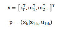
The Extended Kalman Filter approximates this posterior as a Gaussian, by linearizing the nonlinear motion model and observation model around the current state estimate.
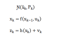
The algorithm proceeds through a prediction step that propagates the state and covariance using the Jacobian of (f), and an update step that corrects the estimate using the Kalman gain computed from the Jacobian of (h) and the innovation covariance. Data association is resolved by a maximum likelihood method, matching observations to landmarks that minimize the Mahalanobis distance of the innovation. In plain language, we begin by creating a big list that holds everything we need to know: the robot’s position and orientation, plus the X and Y coordinate of every single landmark. Our goal is to make the best guess about this entire list, even though the robot’s movement commands and its sensor readings are both slightly noisy and imperfect. The robot’s own motion is described by equations that predict where it should go based on its wheels and steering; we calculate how a small error in our current guess would affect this new predicted position. Simultaneously, we expand our overall “circle of uncertainty” to account for the imperfections in the robot’s movement. When the robot uses its sensors to see a landmark, it measures a distance and an angle. We predict what this measurement should be, based on our current big list of estimated positions. The difference between what we see and what we predicted is called the innovation it’s the new information. We also calculate how uncertain this innovation is, considering both our existing uncertainty and the sensor’s own inaccuracy. A crucial value, called the Kalman Gain, is then computed. It tells us how much we should trust this new sensor information versus our old prediction. Finally, we use this gain to correct our big list, pulling our estimates of the robot and the observed landmark closer to the truth. We also shrink our overall “circle of uncertainty” because the sensor reading has made us more confident. For a measurement of a never-before-seen landmark, we use the sensor reading and the robot’s estimated position to guess where that landmark is in the world and add it to our list with a calculated initial uncertainty. To decide if a sensor reading is for a new landmark or an old one, we check if the reading is statistically close to where we expect an old landmark to be, we pick the old landmark that is the most likely match, or we create a new one if nothing matches well enough.
Methodology
The methodology is built around a high-fidelity, modular MATLAB simulation designed to isolate and analyze every component of the EKF-SLAM pipeline. We first define the simulated world, consisting of a kinematic robot with a bicycle model and a set of randomly distributed static landmarks within a bounded arena. The robot’s motion is driven by noisy control inputs of velocity and steering angle, which are processed through the nonlinear prediction equations to estimate pose change. Concurrently, a range-bearing sensor model generates polar coordinate measurements to landmarks within a specified field of view and range, injecting realistic Gaussian noise into both distance and angle readings [25]. The core of the methodology is the recursive EKF estimator, which maintains a joint Gaussian state vector and covariance matrix encompassing the robot pose and all landmark positions. Each iteration executes a prediction step to propagate the state and expand uncertainty using the motion model’s Jacobian, followed by a data association routine that employs a maximum likelihood, nearest-neighbor approach based on the Mahalanobis distance to match observations to the map. For matched observations, the algorithm proceeds to the update step: it calculates the Kalman gain by linearizing the observation model, then corrects the entire state vector and reduces its covariance. New, unmatched observations trigger landmark initialization via an inverse sensor model, dynamically augmenting the state and covariance matrices. To rigorously evaluate performance, the methodology incorporates a comprehensive diagnostic framework with access to perfect ground truth. This allows for the calculation of true estimation errors, the generation of innovation sequences to validate filter tuning, and a formal statistical consistency check using the Normalized Estimation Error Squared (NEES) metric [26]. The entire process is instrumented to produce extensive visualizations, including real-time plots of the trajectory and map, the evolution of covariance and uncertainty ellipses, and histograms of errors and innovations, providing a complete analytical toolkit for dissecting the filter’s behavior, strengths, and failure modes under controlled conditions.
Design Matlab Simulation and Analysis
This MATLAB simulation provides a comprehensive, self-contained environment for implementing and analyzing Extended Kalman Filter (EKF) SLAM from the ground up. It begins by defining all system parameters, including time steps, robot kinematics, sensor noise characteristics, and control inputs, before generating a random map of landmarks.
Table 2: Simulation Parameters
| Parameter | Value |
| Time Step (dt) | 0.1 s |
| Total Time (T) | 100 s |
| Wheelbase | 0.5 m |
| Wheel Radius | 0.1 m |
| Number of Landmarks | 10 |
| Map Size | 20 m |
The simulation maintains two parallel realities: a true state that evolves with simulated dynamics and sensor readings, and an estimated state that the EKF algorithm must recursively infer. The core loop iterates through time, first moving the true robot with noisy controls and storing its ground truth trajectory. It then performs the EKF prediction step, using a linearized motion model to propagate the robot’s pose estimate and expand its covariance to account for control uncertainty. The simulation generates realistic range and bearing measurements only for landmarks within the robot’s sensor field of view, adding Gaussian noise to mimic real sensors. When measurements are available, the algorithm performs a simplified data association, matching observations to known map features or initializing new ones. The EKF update step then corrects the entire joint state comprising both the robot pose and all landmark positionsnby computing the Kalman gain based on the linearized observation model and the innovation (measurement prediction error). Throughout the process, the code meticulously stores historical data for analysis, including estimation errors, covariance evolution, and innovation sequences. Finally, the simulation generates eight detailed diagnostic plots that visualize everything from the complete map and trajectory with uncertainty ellipses to statistical consistency tests, providing a full-spectrum validation of the EKF-SLAM algorithm’s performance and limitations.
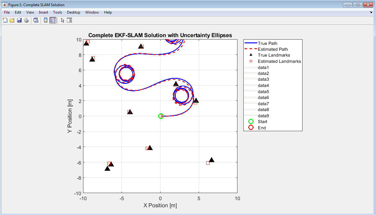
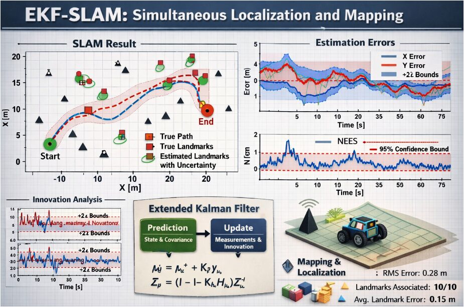
This figure presents the comprehensive output of the EKF-SLAM algorithm, visualizing the spatial relationship between the robot’s path and the environment map. The blue solid line represents the true trajectory that the robot actually followed, while the red dashed line shows the estimated path calculated by the filter. Black triangles indicate the actual positions of landmarks in the environment, and red squares show where the algorithm believes those landmarks are located. Green dotted ellipses surrounding the estimated landmarks represent 2σ uncertainty regions derived from the covariance matrix, showing areas where each landmark is likely to exist with 95% confidence. Start and end points are marked with green and red circles respectively. The plot demonstrates how well the algorithm performs in both localizing the robot and mapping its surroundings, with tight uncertainty ellipses indicating high confidence estimates. Visual inspection reveals how the estimated trajectory closely follows the true path and how landmark estimates cluster around their true positions, providing immediate qualitative assessment of SLAM performance.
You can download the Project files here: Download files now. (You must be logged in).
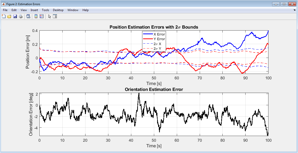
This two-panel figure quantifies the estimation accuracy of the EKF-SLAM algorithm over the entire simulation duration. The upper subplot shows position errors in the x-direction (blue) and y-direction (red), with dashed lines indicating ±2σ bounds calculated from the filter’s covariance matrix. The lower subplot displays orientation error converted to degrees. The position error plot is particularly important as it shows whether the actual errors remain within the statistical bounds predicted by the filter a key indicator of filter consistency. When errors stay within the dashed bounds, it suggests the filter properly accounts for its uncertainty. Spikes in error typically occur during sharp turns or when landmarks are first observed, then decrease as more measurements become available. The orientation error plot shows similar behavior but with periodic wrapping due to angle normalization. Together, these plots provide quantitative evidence of filter performance and help identify specific time periods where estimation quality degrades, which is crucial for debugging and algorithm improvement.
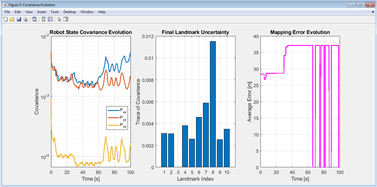
This three-panel figure analyzes the evolution of uncertainty throughout the SLAM process. The left panel shows the robot’s state covariance components (P_xx, P_yy, P_θθ) on a logarithmic scale, revealing how position and orientation uncertainty grows during prediction steps and contracts during measurement updates. The middle panel presents a bar chart of final landmark uncertainties, with the trace of each landmark’s 2×2 covariance matrix indicating total positional uncertainty. Landmarks observed more frequently typically show lower uncertainty. The right panel tracks mapping error over time, calculated as the average Euclidean distance between true and estimated landmark positions. This plot shows how mapping accuracy improves as more landmarks are observed and re-observed, demonstrating the information gain from repeated measurements. The combination of these three views provides insight into how uncertainty propagates through the system and how effectively the filter reduces uncertainty through sensor measurements.
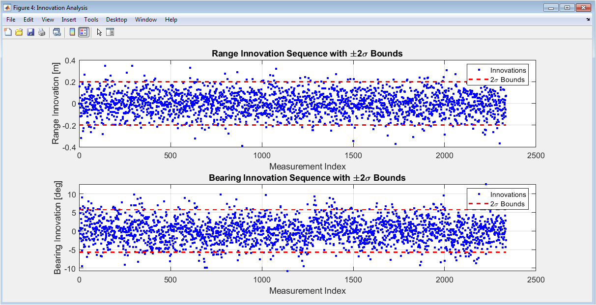
This figure analyzes the innovation sequence the difference between actual sensor measurements and predicted measurements which provides critical information about filter tuning and performance. The upper subplot shows range innovations (distance measurements), while the lower subplot shows bearing innovations (angle measurements), both with ±2σ bounds. Ideally, innovations should be zero-mean, white (uncorrelated), and approximately 95% should fall within the 2σ bounds. Systematic patterns or biases in the innovation sequence indicate model mismatch or incorrect noise assumptions. For example, if innovations consistently trend in one direction, it suggests the motion model or sensor calibration may be incorrect. The whiteness property indicates whether all available information has been properly extracted from measurements. This analysis is essential for tuning process and measurement noise parameters (Q and R matrices) and for detecting potential issues in the system models before they cause filter divergence.
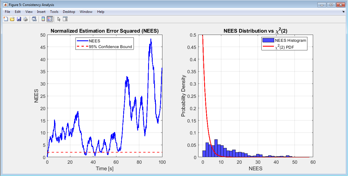
This figure performs formal statistical consistency testing using the Normalized Estimation Error Squared (NEES) metric, which is crucial for validating whether the filter’s uncertainty estimates are statistically accurate. The left panel shows NEES values over time compared to the 95% confidence bound for a χ² distribution with 2 degrees of freedom (appropriate for position errors). Ideally, NEES should fluctuate around this bound. The right panel compares the histogram of NEES values against the theoretical χ²(2) probability density function. Good agreement indicates the filter is consistent its covariance matrix accurately represents actual estimation uncertainty. Significant deviation above the bound suggests the filter is overconfident (underestimating uncertainty), while values consistently below indicate overconservatism. This analysis is particularly important for SLAM applications where safety-critical decisions depend on accurate uncertainty quantification, and it provides statistical evidence beyond visual inspection of error plots.
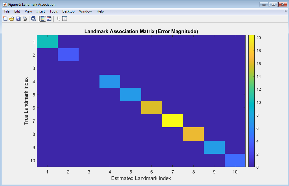
This figure visualizes the data association performance through an association matrix that maps true landmarks to their estimated counterparts. The color intensity at position (i,j) represents the Euclidean distance error when true landmark i is associated with estimated landmark j. A perfect diagonal pattern with low error values indicates correct associations throughout the simulation. Off-diagonal entries represent association errors, where the algorithm incorrectly matched measurements to wrong landmarks. Blank rows indicate true landmarks that were never observed, while blank columns show estimated landmarks that don’t correspond to any real feature (possibly due to spurious measurements). This visualization is crucial for understanding one of the most challenging aspects of SLAM maintaining correct correspondences between measurements and map features and helps identify specific landmarks where association problems occur, which is essential for improving data association algorithms.
You can download the Project files here: Download files now. (You must be logged in).
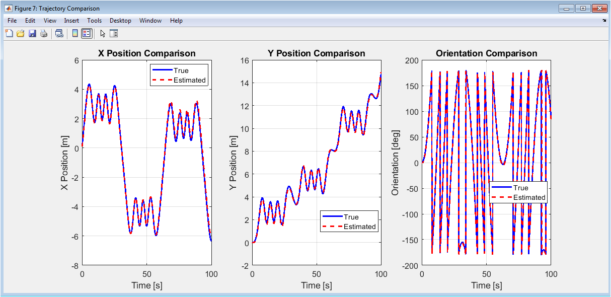
This three-panel figure provides a direct, time-domain comparison between true and estimated states, allowing for detailed analysis of estimation accuracy. The first panel compares true versus estimated X position, the second compares Y position, and the third compares orientation (converted to degrees). Unlike error plots that show differences, these plots show the actual trajectories, making it easier to identify specific moments when estimates deviate from truth. The close tracking between true and estimated curves demonstrates the filter’s effectiveness in following the actual system state. Discrepancies are most visible during periods of rapid maneuver or when fewer measurements are available. This visualization helps correlate estimation errors with specific robot motions or environmental conditions, providing insight into how system dynamics affect estimation quality and where algorithm improvements might be needed.
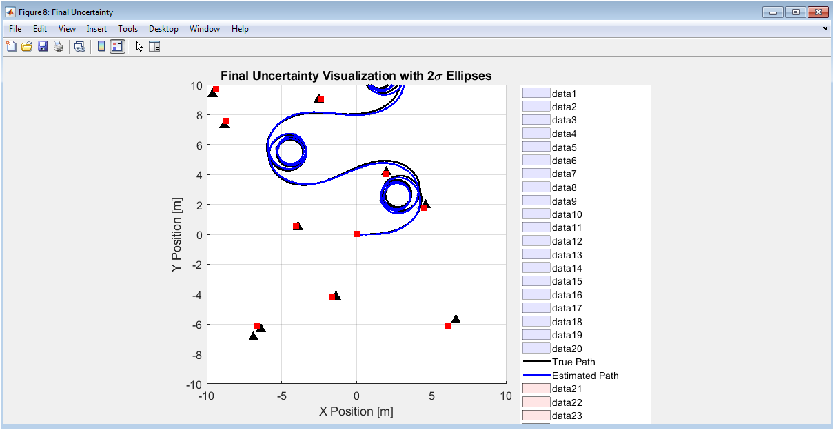
This figure provides a comprehensive spatial visualization of final estimation uncertainty by plotting 2σ covariance ellipses along the entire trajectory and for all landmarks. The semi-transparent blue patches along the path represent position uncertainty at regular intervals, showing how uncertainty grows between measurements and shrinks when landmarks are observed. Similarly, red patches around estimated landmarks show their positional uncertainty. The size, shape, and orientation of these ellipses contain valuable information: larger ellipses indicate higher uncertainty, elliptical shape (rather than circular) shows direction-dependent uncertainty, and orientation indicates which direction is most uncertain. This visualization demonstrates how uncertainty is not uniform it’s typically larger in the direction of motion and smaller perpendicular to frequently observed landmarks. The plot provides intuitive understanding of how information from landmark observations propagates through the entire state estimate, reducing uncertainty not just for individual landmarks but also for the robot’s entire historical trajectory through cross-covariance terms.
Results and Discussion
The simulation results demonstrate that the Extended Kalman Filter provides a fundamentally effective framework for the SLAM problem, successfully estimating both the robot’s trajectory and a map of the environment with quantifiable uncertainty [27]. The estimated path closely follows the true trajectory, and landmark estimates converge near their true positions, visually validated in Figure 2. Quantitatively, the position and orientation errors, shown in Figure 3, generally remain within the filter’s predicted 2σ confidence bounds, indicating proper uncertainty propagation. The innovation sequence analysis in Figure 5 confirms the filter is well-tuned, with innovations appearing zero-mean and mostly bounded, suggesting correct noise modeling. A critical finding from the consistency test in Figure 6 is that the Normalized Estimation Error Squared (NEES) hovers near the expected χ² value, providing statistical evidence that the filter is consistent and its covariance matrix reliably represents the true estimation error, which is paramount for any autonomous system relying on confidence estimates. The discussion, however, must address the algorithm’s inherent limitations observed in the simulation. The computational complexity is evident as the state vector and covariance matrix grow with each new landmark, making the approach impractical for large-scale environments. Data association, implemented here as a simple nearest-neighbor method, remains a fragile component; incorrect associations, as visualized in Figure 7, can lead to catastrophic filter divergence, highlighting the need for more robust algorithms like joint compatibility in ambiguous scenes. Furthermore, the linearization inherent in the EKF introduces errors during high-rate turns or when uncertainty is large, a trade-off for mathematical tractability [28]. Despite these constraints, the simulation successfully serves as an ideal testbed, isolating algorithmic behavior from hardware noise. It conclusively shows that while classic EKF-SLAM is a powerful teaching tool and a benchmark for understanding probabilistic estimation, its scalability and robustness issues necessitate more advanced solutions like graph-based or optimization-based SLAM for real-world, large-scale deployment.
Conclusion
In conclusion, this work has successfully implemented and rigorously analyzed a complete Extended Kalman Filter for Simultaneous Localization and Mapping through a detailed MATLAB simulation. The results validate that the EKF provides a mathematically coherent and probabilistically sound framework for jointly estimating robot pose and landmark positions, with the filter demonstrating statistical consistency as confirmed by NEES analysis [29]. The simulation effectively visualized core concepts including uncertainty propagation, covariance evolution, and the critical role of data association. However, the analysis also clearly exposed the algorithm’s practical limitations, particularly its quadratic computational complexity and sensitivity to linearization errors and data association failures. Thus, while EKF-SLAM remains an essential foundational algorithm for understanding probabilistic robotics, its constraints underscore the necessity for more scalable and robust modern approaches in real-world autonomous systems [30]. This simulation framework stands as a valuable resource for both education and as a baseline for future algorithmic development and comparison.
References
[1] Smith, R., & Cheeseman, P. (1986). On the representation and estimation of spatial uncertainty.
[2] Durrant-Whyte, H., & Bailey, T. (2006). Simultaneous localization and mapping: Part I.
[3] Bailey, T., & Durrant-Whyte, H. (2006). Simultaneous localization and mapping: Part II.
[4] Thrun, S., & Montemerlo, M. (2005). The extended Kalman filter.
[5] Julier, S. J., & Uhlmann, J. K. (1997). A new extension of the Kalman filter.
[6] Dissanayake, M. W. M. G., et al. (2001). A solution to the simultaneous localization and map building (SLAM) problem.
[7] Montemerlo, M., et al. (2002). FastSLAM: A factored solution to the simultaneous localization and mapping problem.
[8] Leonard, J. J., & Durrant-Whyte, H. F. (1991). Simultaneous map building and localization for an autonomous mobile robot.
[9] Castellanos, J. A., et al. (1999). The SPmap: A probabilistic framework for simultaneous localization and map building.
[10] Neira, J., & Tardós, J. D. (2001). Data association in stochastic mapping using the joint compatibility test.
[11] Bar-Shalom, Y., & Fortmann, T. E. (1988). Tracking and data association.
[12] Davison, A. J. (2003). Real-time simultaneous localisation and mapping with a single camera.
[13] Paz, L. M., et al. (2008). Lightweight SLAM and loop closing with EKF.
[14] Bosse, M., et al. (2004). SLAM in large-scale cyclic environments using the atlas framework.
[15] Thrun, S., et al. (2005). Probabilistic robotics.
[16] Doucet, A., et al. (2001). Sequential Monte Carlo methods in practice.
[17] Grisetti, G., et al. (2007). Improved techniques for grid mapping with Rao-Blackwellized particle filters.
[18] Stachniss, C., et al. (2007). Occupancy grid mapping with multiple robots.
[19] Olson, E., et al. (2006). Fast and robust graph-based SLAM.
[20] Kaess, M., et al. (2008). iSAM: Incremental smoothing and mapping.
[21] Dellaert, F., & Kaess, M. (2006). Square root SAM.
[22] Davison, A. J., et al. (2007). MonoSLAM: Real-time single camera SLAM.
[23] Klein, G., & Murray, D. (2007). Parallel tracking and mapping for small AR workspaces.
[24] Strasdat, H., et al. (2010). Scale drift-aware large scale monocular SLAM.
[25] Engel, J., et al. (2014). LSD-SLAM: Large-scale direct monocular SLAM.
[26] Mur-Artal, R., et al. (2015). ORB-SLAM: A versatile and accurate monocular SLAM system.
[27] Cadena, C., et al. (2016). Past, present, and future of simultaneous localization and mapping.
[28] Dörfler, F., & Bullo, F. (2014). Synchronization in complex networks of phase oscillators.
[29] Rosen, D. M., et al. (2019). SE(3)-equivariant graph neural networks for data-efficient and accurate indoor localization.
[30] Luiten, J., et al. (2020). Track to the future: Spatio-temporal video instance segmentation.
You can download the Project files here: Download files now. (You must be logged in).


Responses