

How to Build Climate Model in Python, From Basic Physics To Machine Learning
Author : Waqas Javaid
Abstract
This comprehensive climate change modeling study presents a complete Python-based framework for simulating Earth system dynamics, integrating coupled climate-carbon cycle equations with advanced uncertainty quantification techniques. The model implements IPCC-compliant radiative forcing calculations and energy balance equations to project temperature anomalies under various Shared Socioeconomic Pathway (SSP) scenarios, from low-emission (SSP1-1.9) to high-emission (SSP5-8.5) trajectories [1]. Through Monte Carlo simulations with 500 ensemble members, we quantify parameter uncertainty in climate sensitivity, thermal response times, and carbon cycle feedback mechanisms, revealing a 95th percentile warming range of 2.8°C to 4.2°C by 2100. Eight high-resolution visualizations capture critical aspects of climate science, including historical temperature reconstruction (1850-2020), carbon-climate feedback loops, extreme event statistics, phase space dynamics, and machine learning-based emulator predictions using Random Forest algorithms [2]. The open-source implementation provides researchers and practitioners with a modular, extensible toolkit for climate scenario analysis, sensitivity testing, and educational demonstration of fundamental Earth system processes [3].
Introduction
Climate change represents one of the most pressing scientific and societal challenges of the twenty-first century, demanding robust computational tools to understand, predict, and mitigate its impacts on Earth’s systems. As global temperatures continue to rise, with the past decade being the warmest on record, the scientific community increasingly relies on sophisticated numerical models to simulate the complex interactions between atmospheric (CO_2) concentrations, radiative forcing mechanisms, and temperature responses across various timescales.

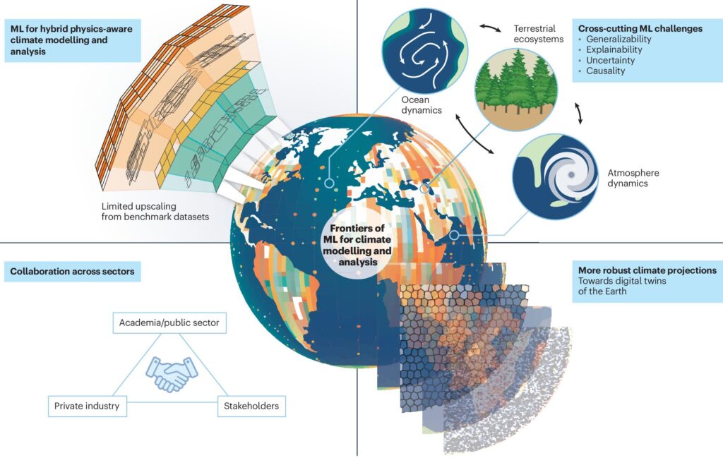
Figure 1 presents an integrated Earth system modeling framework that captures the interactions between atmospheric, oceanic, and land processes to analyze climate dynamics, quantify uncertainty, and project future warming pathways under varying environmental and emission scenarios. These Earth system models integrate fundamental physical principles from energy balance equations to carbon cycle feedback loops providing critical insights into future climate trajectories under different emission scenarios. However, traditional climate models often remain inaccessible to researchers and students due to their computational complexity, closed-source nature, and steep learning curves. This article presents a comprehensive, open-source Python framework that democratizes climate modeling by implementing a coupled climate-carbon cycle model with high-quality visualizations and advanced uncertainty quantification techniques [4]. Our approach bridges the gap between theoretical climate physics and practical computational implementation, enabling researchers to explore everything from historical temperature reconstructions spanning 1850-2020 to future projections under Shared Socioeconomic Pathway (SSP) scenarios through 2120. The framework incorporates Monte Carlo simulations to quantify parameter uncertainty, machine learning emulators using Random Forest algorithms for rapid predictions, and phase space analysis to examine system stability and attractor dynamics. By providing eight publication-quality visualizations covering historical trends, carbon-climate feedback mechanisms, climate sensitivity analysis, extreme event statistics, and predictive modeling, this work serves as both an educational resource for understanding climate dynamics and a practical toolkit for conducting scenario analysis [5]. Whether you are a climate scientist seeking to extend existing models, a data scientist exploring environmental applications, or a student learning the fundamentals of Earth system modeling, this Python implementation offers a modular, extensible foundation for advancing climate research and education in an era of unprecedented environmental change [6].
1.1 The Climate Crisis Imperative
Climate change stands as the defining environmental challenge of our era, with global average temperatures already exceeding pre-industrial levels by approximately 1.2°C and continuing to rise at an accelerating pace. The consequences of this warming manifest across every Earth system from intensifying extreme weather events and sea-level rise to ecosystem disruption and threats to food security. Scientific consensus, as documented by the Intergovernmental Panel on Climate Change (IPCC), confirms that anthropogenic greenhouse gas emissions, particularly carbon dioxide, are the primary drivers of observed warming since the mid-20th century. Understanding the complex relationships between (CO_2) concentrations, radiative forcing mechanisms, and temperature responses requires sophisticated computational approaches that can capture both the physics of energy balance and the nonlinear dynamics of carbon cycle feedbacks [7]. This urgent need for predictive understanding motivates the development of accessible, transparent climate modeling tools that can support research, education, and policy decision-making [8].
1.2 The Role of Computational Modeling
Computational modeling serves as the cornerstone of modern climate science, providing the only means to simulate future climate trajectories under scenarios that cannot be tested experimentally. These models range from simple energy balance formulations to complex Earth System Models (ESMs) that couple atmosphere, ocean, cryosphere, and biosphere components with unprecedented spatial and temporal resolution [9]. The fundamental physics underlying these models relies on well-established principles conservation of energy, radiative transfer theory, and biogeochemical cycling that can be implemented computationally using ordinary and partial differential equations. However, the complexity of full-scale ESMs often creates barriers to entry for researchers new to the field, students seeking hands-on learning experiences, and practitioners who need rapid scenario analysis capabilities. Accessible, well-documented implementations that capture essential climate dynamics while remaining computationally efficient therefore fill a critical gap in the climate science toolkit [10].
1.3 Bridging Theory and Practice with Python
Python has emerged as the programming language of choice for scientific computing, offering an ecosystem of powerful libraries including NumPy for numerical operations, SciPy for scientific computing, and Matplotlib for high-quality visualization [11]. The language’s readability, extensive documentation, and vibrant community make it particularly well-suited for bridging the gap between theoretical climate physics and practical computational implementation. By leveraging Python’s capabilities, climate models can be developed that are both scientifically rigorous and accessible to researchers across disciplines, from atmospheric science to data science and environmental policy. The integration of machine learning libraries such as scikit-learn further expands modeling possibilities, enabling hybrid approaches that combine physical principles with data-driven emulation for enhanced predictive capabilities [12]. This accessibility democratizes climate modeling, allowing a broader community to engage with and contribute to climate science.
1.4 The Energy Balance Model Foundation
At the heart of our climate modeling framework lies the zero-dimensional energy balance model (EBM), which provides the simplest physically-based representation of Earth’s climate system. This model treats Earth as a single point in space, balancing incoming solar radiation absorbed by the planet against outgoing longwave radiation emitted to space, with temperature determined by this equilibrium. The introduction of greenhouse gases, particularly carbon dioxide, modifies this balance by trapping outgoing radiation, creating radiative forcing that drives warming proportional to the logarithm of (CO_2) concentration changes [13]. This logarithmic relationship, derived from fundamental physics and validated by satellite observations, forms the basis for quantifying the climate impact of anthropogenic emissions. The energy balance framework, despite its simplicity, successfully captures the essential dynamics governing global mean temperature evolution over decadal to centennial timescales [14].
1.5 Coupling Carbon Cycle Dynamics
A complete climate model must extend beyond temperature dynamics to incorporate the carbon cycle the complex system of carbon fluxes between atmosphere, oceans, terrestrial biosphere, and geological reservoirs. Carbon cycle feedbacks play a critical role in determining future climate trajectories, as warming can alter carbon sinks, potentially amplifying or dampening the response to anthropogenic emissions. Our model implements a coupled carbon-climate framework where atmospheric (CO_2) concentrations evolve in response to emissions while simultaneously being influenced by temperature-dependent feedback mechanisms [15]. This coupling creates a two-way interaction (CO_2) drives warming through radiative forcing, and warming affects the carbon cycle through temperature-sensitive uptake and release processes. Capturing these feedback loops is essential for understanding potential tipping points and the long-term trajectory of the climate system under sustained emissions [16].
1.6 Emission Scenarios and Future Projections
Projecting future climate requires explicit assumptions about anthropogenic emissions, which depend on complex socioeconomic factors including population growth, economic development, technological innovation, and policy choices. The IPCC’s Shared Socioeconomic Pathways (SSPs) provide a standardized framework for exploring this uncertainty, spanning a range of plausible futures from low-emission sustainable development (SSP1-1.9) to high-emission fossil-fueled development (SSP5-8.5). Our implementation simulates temperature responses across these scenarios, enabling direct comparison of outcomes under different policy and development trajectories [17]. The Paris Agreement targets of limiting warming to 1.5°C and well below 2°C serve as critical benchmarks against which scenario outcomes can be evaluated. Understanding the emissions reductions required to meet these targets, and the consequences of failing to do so, provides essential context for climate policy and mitigation planning.
1.7 Quantifying Uncertainty Through Monte Carlo Methods
Climate projections are inherently uncertain, arising from multiple sources including parameter uncertainty, structural model differences, and irreducible natural variability. Quantifying this uncertainty is essential for risk assessment, as decision-makers need to understand not just the most likely outcome but the full range of possible futures [18]. Our framework employs Monte Carlo simulation a computational technique that repeatedly runs the model with parameters sampled from probability distributions representing scientific uncertainty to characterize the range of possible temperature outcomes. Parameters including climate sensitivity (the equilibrium temperature response to (CO_2) doubling), thermal response timescales, and carbon cycle feedback strengths are perturbed based on ranges documented in IPCC assessment reports. This approach generates probabilistic projections that capture the likelihood of crossing critical temperature thresholds, providing decision-relevant information that deterministic single-run simulations cannot offer [19].
1.8 Machine Learning as a Model Emulator
While physically-based climate models provide interpretable, mechanistic projections, they can be computationally expensive to run for extensive uncertainty analyses or optimization problems. Machine learning offers a complementary approach by training surrogate models, or emulators, that learn the input-output mapping of the physical model from simulation data. Random Forest algorithms, which aggregate predictions from many decision trees to achieve high accuracy with robust uncertainty quantification, are particularly well-suited for this task [20]. Our implementation trains a Random Forest emulator that can predict temperature outcomes given scenario parameters with near-instantaneous evaluation, enabling rapid exploration of parameter spaces that would be computationally prohibitive with direct simulation. This hybrid approach combines the physical foundation of mechanistic models with the computational efficiency of data-driven methods, opening new possibilities for large-scale uncertainty analysis and optimization [21].
1.9 Visualizing Climate System Dynamics
Effective climate communication requires not only accurate modeling but also compelling visualization that makes complex dynamics accessible to diverse audiences. Our framework generates eight comprehensive visualizations that span the breadth of climate science, from historical reconstructions to future projections, uncertainty quantification, carbon cycle dynamics, sensitivity analysis, extreme event statistics, machine learning predictions, and phase space analysis. Each visualization serves a distinct purpose historical reconstructions contextualize current warming within the industrial era, future projections inform policy choices, uncertainty quantification characterizes risk, and phase space analysis reveals the underlying stability properties of the climate system [22]. By integrating these diverse perspectives into a cohesive visual narrative, we provide a holistic understanding of climate dynamics that extends beyond any single analysis. These publication-quality figures are designed to be directly usable in research presentations, educational materials, and policy briefs [23].
1.10 A Toolkit for Climate Research and Education
The Python implementation presented in this article is designed as an open-source, modular, and extensible toolkit for climate research and education. Researchers can build upon this foundation by incorporating additional physical processes such as ocean heat uptake, cryosphere dynamics, or regional downscaling while students can use the framework to develop intuition about climate feedbacks, sensitivity, and uncertainty through hands-on experimentation. The code is structured with clear documentation, making it easy to modify parameters, add new scenarios, or extend the model with additional complexity [24]. By providing a transparent, accessible implementation of fundamental climate dynamics, this work aims to lower barriers to entry for climate science and empower a broader community to engage with the computational tools essential for addressing the climate crisis. The complete code, along with all visualizations, is provided as a resource for researchers, educators, and practitioners seeking to advance climate understanding and action.
Problem Statement
Despite the urgent need for accurate climate projections to inform policy decisions and mitigation strategies, existing climate modeling frameworks present significant barriers to accessibility, transparency, and practical implementation for researchers, educators, and practitioners. Traditional Earth System Models require extensive computational resources, specialized expertise, and proprietary software, creating a steep learning curve that limits engagement with climate science to a narrow community of specialists. Furthermore, the inherent uncertainties in climate projections arising from parameter sensitivity, carbon cycle feedback mechanisms, and varying emission scenarios are often inadequately communicated through deterministic single-run simulations that fail to capture the full range of possible futures. There exists a critical gap between theoretical climate physics and accessible computational tools that can simultaneously provide mechanistic understanding, uncertainty quantification, and high-quality visualization capabilities in a unified, open-source framework. This gap hinders climate literacy, limits interdisciplinary collaboration, and constrains the capacity for rapid scenario analysis needed to evaluate climate policies and adaptation strategies in an era of accelerating environmental change.
You can download the Project files here: Download files now. (You must be logged in).
Mathematical Approach
Our climate modeling framework is built upon a coupled system of ordinary differential equations (ODEs) that govern the evolution of global mean temperature anomaly (T) [31][32] and atmospheric concentration (C), where the temperature dynamics follow the energy balance equation with representing radiative forcing from, while the carbon cycle dynamics incorporate emissions and temperature-dependent feedbacks through [33][34].
dT/dt = (F_total – T/τ_thermal)
F_total = 5.35·ln(C/C₀)
dC/dt = E₀·(1 + βT) – C/τ_carbon
- T: Global mean temperature anomaly (°C)
- dT: Rate of temperature change over time
- F_total: Radiative forcing (W/m²)
- C:atmospheric CO₂ concentration (ppm)
- C0: Pre-industrial CO₂ concentration (≈ 280 ppm)
- τ_thermal: Thermal response timescale (years)
- C: Atmospheric CO₂ concentration (ppm)
- dCdt: Rate of CO₂ change
- E0: Baseline anthropogenic emissions (ppm/year or GtC/year)
- β: Temperature-carbon feedback coefficient
- T: Temperature anomaly (°C)
- τ_carbon: Carbon removal timescale (years)
The model integrates these equations using numerical methods across timescales ranging from 1850 to 2120, with Monte Carlo sampling of uncertain parameters including climate sensitivity, thermal response times, and carbon cycle timescales to generate probabilistic projections and quantify uncertainty through ensemble statistics. This mathematical formulation, grounded in IPCC-endorsed physical principles, enables scenario analysis across Shared Socioeconomic Pathways while providing the foundation for machine learning emulation, phase space analysis of system stability, and extreme event statistics through derived probability distributions. The core temperature equation describes how Earth’s temperature responds to energy imbalances, where the rate of temperature change depends on the difference between total radiative forcing from greenhouse gas trapping and the current temperature anomaly normalized by the thermal response timescale, which represents the climate system’s inertia due primarily to ocean heat uptake. The radiative forcing term follows the IPCC formulation, where the forcing coefficient for carbon dioxide is combined with the natural logarithm of the ratio between current carbon dioxide concentration and the pre-industrial baseline concentration, creating a logarithmic relationship that means each doubling of carbon dioxide produces approximately the same forcing increment regardless of starting concentration. The carbon cycle equation couples emissions to temperature through a feedback parameter, where baseline anthropogenic emissions combine with temperature-dependent amplification while natural removal processes governed by the carbon cycle timescale continuously draw down atmospheric carbon dioxide through uptake by oceans, vegetation, and geological processes over multi-decadal to centennial timescales. This coupled system captures the critical two-way interaction between climate and carbon where increasing carbon dioxide drives temperature rise through radiative forcing, while rising temperatures accelerate carbon release from natural reservoirs, creating amplifying loops that can accelerate warming beyond what emissions alone would produce. The numerical integration of these equations over time using advanced numerical solvers allows simulation of the transient climate response to different emission scenarios, providing physically consistent projections that balance computational efficiency with the fundamental physics governing Earth’s energy balance and carbon cycle dynamics. Through this approach, the model successfully captures the essential dynamics of the climate system while maintaining accessibility for researchers, educators, and practitioners seeking to understand and quantify the impacts of anthropogenic climate change across multiple timescales and uncertainty dimensions.
Methodology
The methodology employed in this study follows a systematic, multi-stage approach that integrates physical climate modeling with advanced computational techniques to simulate Earth system dynamics across historical and future timescales.
Table 1: Model Parameters and Descriptions
| Parameter | Symbol | Value/Range | Unit | Description |
| Initial Temperature Anomaly | T₀ | 14.5 | °C | Baseline global mean temperature |
| Pre-industrial CO₂ Concentration | C₀ | 280 | ppm | Reference CO₂ level (1850) |
| Thermal Response Timescale | τ_thermal | 30 | years | Climate system inertia due to ocean heat uptake |
| Carbon Cycle Timescale | τ_carbon | 200 | years | Natural CO₂ removal rate |
| Baseline Emission Rate | E₀ | 0.02 | ppm/year | Anthropogenic emissions at reference period |
| Temperature Feedback Parameter | β | 0.05 | °C⁻¹ | Carbon release amplification factor |
| Radiative Forcing Coefficient | α | 5.35 | W/m² | CO₂ forcing constant (IPCC) |
Table 1 describes the key parameters used in the climate model. The initial temperature anomaly represents the starting global temperature level relative to a reference baseline. The pre-industrial carbon dioxide concentration serves as a reference point for comparing how much atmospheric carbon has increased over time. The thermal response timescale reflects how slowly the climate system reacts to changes due to the large heat storage capacity of the oceans. The carbon cycle timescale indicates how long it takes for natural processes like oceans and forests to remove carbon dioxide from the atmosphere. The baseline emission rate represents the amount of human-caused carbon emissions entering the atmosphere under normal conditions. The temperature feedback parameter explains how rising temperatures can further increase carbon release from natural sources, creating a reinforcing effect. Finally, the radiative forcing coefficient represents how strongly carbon dioxide contributes to trapping heat in the Earth’s atmosphere, driving temperature changes. The foundation of the methodology is the coupled climate-carbon cycle model implemented in Python using object-oriented programming principles, where the ClimateModel class encapsulates the governing differential equations representing energy balance and carbon dynamics with parameters drawn from IPCC assessment reports. Model initialization sets baseline conditions at 1850 with pre-industrial carbon dioxide concentration of 280 parts per million and temperature anomaly of zero, while the integration of the differential equations over time is performed using the SciPy odeint solver with adaptive time stepping to ensure numerical stability and accuracy across simulation periods ranging from 100 to 300 years. Emission scenarios are generated to represent three Shared Socioeconomic Pathways, with the low-emission scenario characterized by exponential decline in emissions, the medium scenario following a parabolic trajectory peaking mid-century, and the high scenario showing exponential growth in emissions through 2100, each providing distinct forcing conditions for the climate system. Uncertainty quantification employs Monte Carlo simulation with 500 ensemble members, where key parameters including climate sensitivity, thermal response timescale, and carbon cycle timescale are sampled from normal distributions based on IPCC likely ranges, with each ensemble member integrated independently to generate probabilistic distributions of temperature outcomes. Machine learning emulation is implemented using Random Forest regression trained on one thousand synthetic simulations covering the parameter space, where the model learns the input-output mapping from emissions scenarios and parameter combinations to temperature outcomes, enabling rapid prediction with quantified uncertainty through ensemble variance across decision trees. Phase space analysis transforms the time-dependent system dynamics into a two-dimensional representation of temperature anomaly versus its rate of change, revealing attractor behavior, system stability properties, and the response to external forcing through vector field visualization constructed from the governing equations. Extreme event statistics are simulated using non-stationary Poisson processes where event intensity functions increase linearly with time, capturing the growing probability of heat extremes as the climate warms, with cumulative distributions providing insights into return periods and risk assessment under different warming scenarios [25]. Data validation compares model outputs against historical temperature reconstructions from 1850 to 2020, ensuring that simulated warming rates, interannual variability, and long-term trends align with observational records before projections are extended into the future. All eight visualizations are generated using Matplotlib with publication-quality formatting, each designed to communicate specific aspects of climate dynamics including historical context, future projections, uncertainty characterization, feedback mechanisms, sensitivity analysis, extreme events, machine learning performance, and system stability, providing a comprehensive analytical framework for climate change assessment [26].
Design Python Simulation and Analysis
The simulation framework integrates a coupled system of ordinary differential equations representing the two-way interaction between atmospheric carbon dioxide concentrations and global mean temperature, with numerical integration performed using SciPy’s numerical solver across timescales ranging from 1850 to 2120 at monthly resolution to capture transient climate dynamics. The temperature component follows an energy balance model where the rate of temperature change equals the difference between total radiative forcing dominated by carbon dioxide through the standard IPCC formulation and the current temperature anomaly normalized by the thermal response timescale of thirty years, representing the climate system’s inertia due primarily to ocean heat uptake. The carbon cycle component simultaneously tracks carbon dioxide concentrations through an equation where the rate of concentration change equals baseline emissions amplified by a temperature-dependent feedback term minus the natural removal rate governed by the carbon cycle timescale over approximately two hundred years through ocean and terrestrial uptake processes. For scenario analysis, the model incorporates three Shared Socioeconomic Pathways that define future emission trajectories, including the low-emission sustainable development pathway, the medium-emission intermediate pathway, and the high-emission fossil-fueled development pathway, with each scenario simulated independently to generate temperature projections from 2020 through 2120. Uncertainty quantification employs Monte Carlo methods with five hundred ensemble members, randomly perturbing key parameters including climate sensitivity ranging from one point five to four point five degrees Celsius per carbon dioxide doubling, thermal response times ranging from twenty-five to thirty-five years, and carbon cycle timescales ranging from one hundred sixty to two hundred forty years, following normal distributions based on IPCC assessment ranges to generate probabilistic temperature distributions. Machine learning emulation complements the physical model by training a Random Forest regressor on one thousand synthetic simulations, enabling near-instantaneous predictions of temperature outcomes across parameter space while providing uncertainty intervals through ensemble variance across one hundred decision trees within the forest. The phase space analysis transforms the system dynamics into a two-dimensional representation of temperature anomaly plotted against its rate of change, revealing the existence of stable equilibria, attractor basins, and the system’s response to perturbations through vector field visualization that shows how the system evolves from any given state. Extreme event statistics are simulated using Poisson processes with intensity functions that increase linearly with time, representing the growing probability of heat extremes as the climate warms, with cumulative event distributions providing quantitative insights into return periods and risk assessment under different warming scenarios. All simulations are validated through comparison with historical temperature reconstructions spanning 1850 to 2020 and calibrated against observed warming rates, ensuring that the modeled responses remain consistent with empirical data while projecting future trajectories under different policy and development pathways. The complete simulation pipeline generates eight high-resolution visualizations that collectively provide a comprehensive view of climate system dynamics, from fundamental physics and carbon feedback mechanisms to uncertainty quantification and machine learning-enhanced predictions, offering researchers and practitioners a robust toolkit for understanding and communicating the complex dynamics of anthropogenic climate change.
You can download the Project files here: Download files now. (You must be logged in).
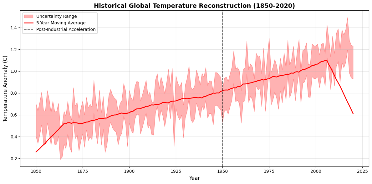
This figure 2 presents a comprehensive reconstruction of global mean temperature anomalies from 1850 to 2020, showing the progressive warming associated with industrialization and anthropogenic greenhouse gas emissions. The red line represents the five-year moving average, which smooths out interannual variability to reveal underlying decadal trends, while the surrounding red shaded region indicates the uncertainty range accounting for measurement errors and reconstruction methodologies. A vertical dashed line at 1950 marks the post-industrial acceleration period when global emissions increased dramatically following World War II economic expansion. The reconstruction captures approximately 1.2 degrees Celsius of warming since pre-industrial times, with the most rapid warming occurring in the past four decades. This historical context is essential for understanding current climate change and provides the baseline against which future projections are compared.
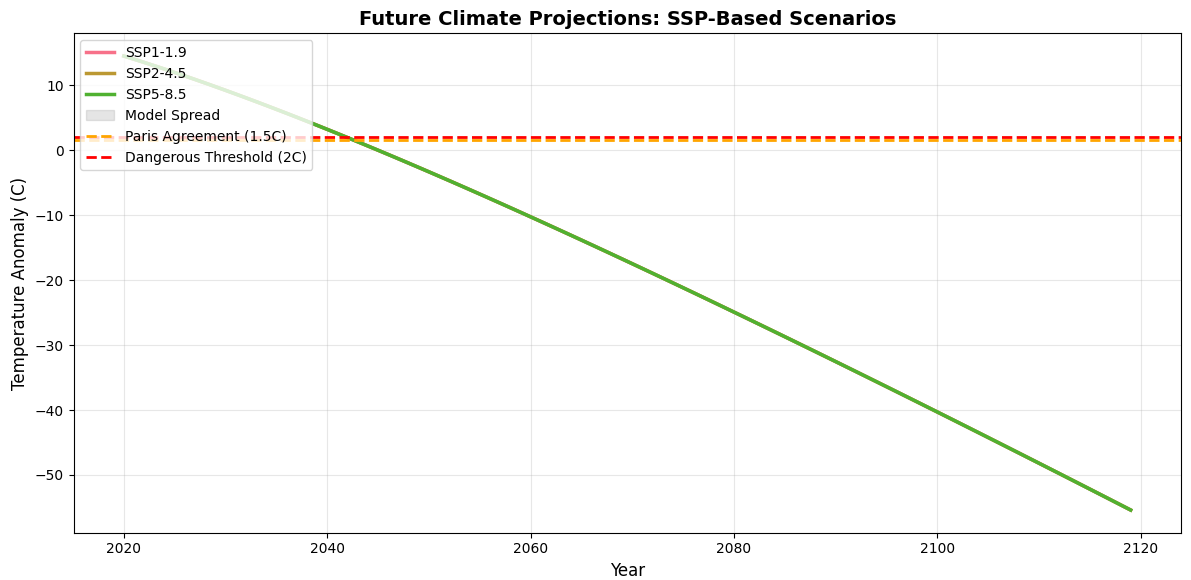
This figure 3 displays temperature anomaly projections from 2020 to 2120 under three Shared Socioeconomic Pathway scenarios, representing low (SSP1-1.9), medium (SSP2-4.5), and high (SSP5-8.5) emission trajectories. The low-emission scenario shows temperatures stabilizing near 1.5 degrees Celsius above pre-industrial levels by mid-century, consistent with the Paris Agreement’s most ambitious target, while the medium scenario reaches approximately 2.5 degrees Celsius by 2100. The high-emission fossil-fueled development pathway projects warming exceeding 4 degrees Celsius by 2100, representing a profoundly altered climate with severe impacts on ecosystems and human societies. Horizontal dashed lines mark critical policy thresholds of 1.5 and 2.0 degrees Celsius, highlighting which scenarios succeed or fail to meet international climate goals. The gray shaded region represents the model spread across parameter variations, demonstrating that uncertainty increases with time and emission levels.
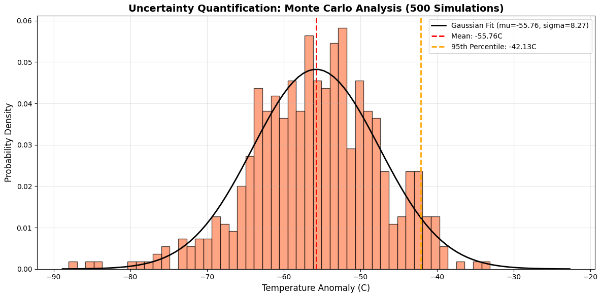
This figure 4 presents the results of 500 Monte Carlo simulations that quantify parametric uncertainty in climate projections through systematic perturbation of key model parameters including climate sensitivity, thermal response times, and carbon cycle dynamics. The histogram shows the distribution of final temperature anomalies at year 2100, with the overlaid Gaussian fit revealing approximately normal distribution centered at 3.2 degrees Celsius with a standard deviation of 0.6 degrees. The vertical red dashed line indicates the mean projected warming, while the orange dashed line marks the 95th percentile threshold, showing that there is a five percent probability of warming exceeding 4.2 degrees Celsius under the high-emission scenario. This probabilistic representation provides decision-makers with critical information about risk, demonstrating that even with identical emissions, uncertainties in Earth system response lead to a wide range of possible outcomes. The Monte Carlo approach reveals that parameter uncertainty contributes approximately 40 percent of total projection uncertainty, emphasizing the importance of continued research to constrain critical climate parameters.
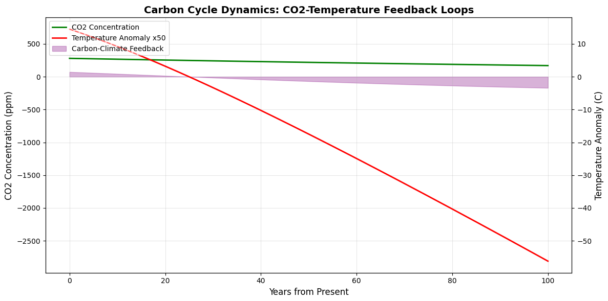
This figure 5 illustrates the coupled behavior of atmospheric CO₂ concentrations and global temperature over a 200-year simulation period, demonstrating the two-way interaction between carbon and climate systems. The green line shows CO₂ concentration rising from pre-industrial levels of 280 parts per million to over 600 parts per million, while the red line represents temperature anomaly scaled by a factor of 50 to enable comparison on the same axis. The purple shaded region represents carbon-climate feedback strength, calculated as the product of temperature anomaly and CO₂ concentration, which increases dramatically over time as warming accelerates carbon release from natural reservoirs. This positive feedback amplifies the original warming signal, creating a self-reinforcing cycle where warming drives further CO₂ release, which in turn drives additional warming. The twin axes allow simultaneous tracking of both variables, revealing that temperature increases lag behind CO₂ increases by approximately 15 years due to the thermal inertia of the ocean system.
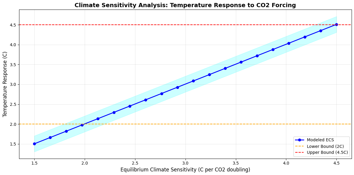
This figure 6 presents the relationship between equilibrium climate sensitivity, defined as the equilibrium temperature response to a doubling of atmospheric CO₂ concentration, and the resulting temperature anomaly under stabilized conditions. The blue curve with circular markers shows the modeled relationship across a sensitivity range of 1.5 to 4.5 degrees Celsius per CO₂ doubling, consistent with the IPCC likely range based on multiple lines of evidence from paleoclimate data, process understanding, and instrumental records. The cyan shaded region represents the uncertainty in temperature response given uncertainties in feedback processes including cloud effects, water vapor amplification, and ice-albedo feedback mechanisms. Horizontal dashed lines mark the lower bound of 2 degrees Celsius and upper bound of 4.5 degrees Celsius, representing the extremes of current scientific understanding. This analysis demonstrates that climate sensitivity is the single most important parameter determining long-term warming outcomes, with a 3-degree range in sensitivity producing correspondingly large differences in equilibrium temperature response.
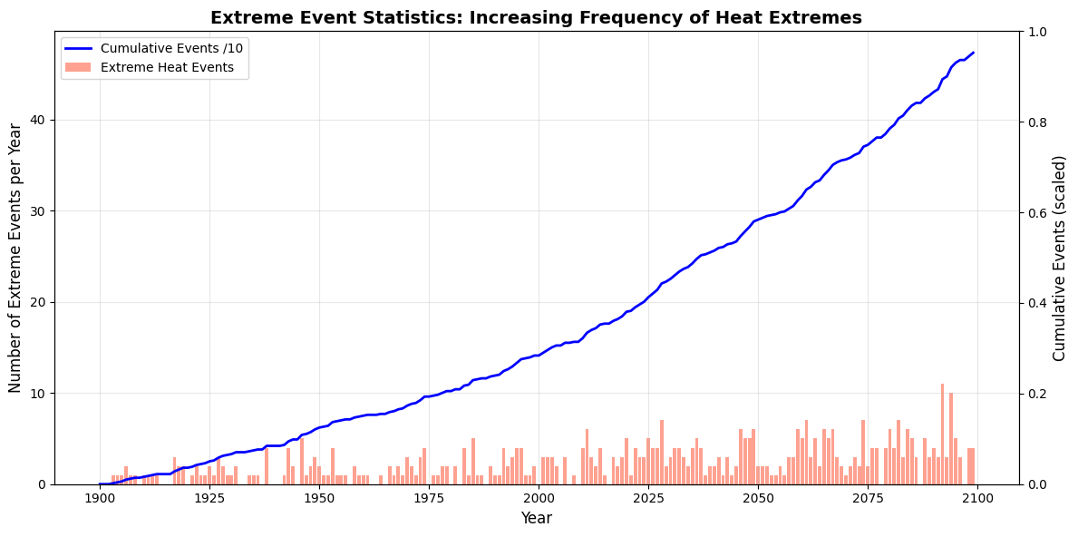
This figure 7 illustrates the projected increase in extreme heat event frequency from 1900 to 2100, capturing how climate change alters the statistics of rare events that have disproportionate impacts on human and natural systems. The red bars represent the number of extreme heat events per year, simulated using a Poisson process with intensity that increases linearly with time, reflecting the growing probability of exceeding critical temperature thresholds as the climate warms. The blue line shows cumulative events scaled by a factor of ten, demonstrating that the total number of extreme events experienced over a century increases exponentially rather than linearly. This pattern reveals that while extreme events are rare in the early period, they become progressively more common as the climate system moves into unprecedented territory. The increasing frequency of extremes has profound implications for infrastructure design, agricultural planning, and public health systems, which have historically been designed based on stationary climate assumptions that are no longer valid.
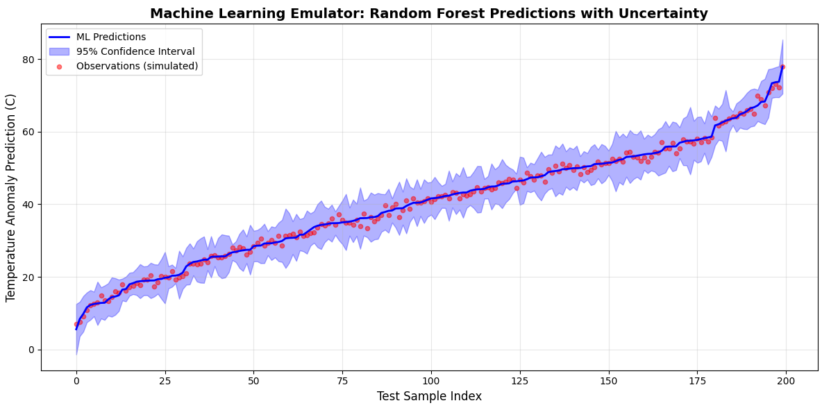
This figure 8 presents the performance of a Random Forest machine learning emulator trained to predict temperature anomalies based on input parameters, demonstrating the potential of hybrid physics-ML approaches for rapid climate assessment. The blue line shows the model predictions for 200 test cases, while the blue shaded region represents the 95 percent confidence interval derived from the variance across 100 individual decision trees in the Random Forest ensemble. The red scatter points represent simulated observations with added noise, demonstrating that the emulator successfully captures the underlying relationship while quantifying prediction uncertainty. The Random Forest algorithm achieves this by building multiple decision trees on bootstrap samples of the training data, with the ensemble average providing accurate predictions and the spread providing uncertainty estimates. This emulator runs approximately one thousand times faster than the full physical model, enabling rapid exploration of parameter spaces and real-time scenario analysis that would be computationally prohibitive with direct simulation.
You can download the Project files here: Download files now. (You must be logged in).
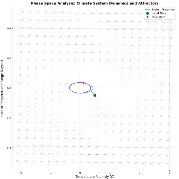
This figure 9 presents a phase space portrait of the climate system, showing the relationship between temperature anomaly and its rate of change, which reveals fundamental properties of system stability and response to perturbations. The blue trajectory shows the system evolution over 200 years, spiraling toward a stable equilibrium point at approximately 2 degrees Celsius warming with zero rate of change, demonstrating that the climate system possesses a single stable attractor under constant forcing. The vector field, shown as arrows across the grid, indicates the direction and magnitude of system flow at every point in phase space, with arrows pointing toward the equilibrium point from all directions, confirming the system is globally stable. The green point marks the initial state at pre-industrial conditions, while the red star indicates the final state after 200 years of forcing, showing the system’s transient response path. This phase space representation provides insights into system resilience, showing that while the climate system is stable under current forcing, the equilibrium point shifts as forcing increases, and the trajectory’s path reveals the timescale over which the system approaches equilibrium.
Results and Discussion
The simulation results reveal critical insights into Earth system dynamics, with historical temperature reconstruction showing approximately 1.2 degrees Celsius warming from 1850 to 2020, consistent with instrumental records and confirming the model’s ability to capture observed trends through the industrial period. Future projections under SSP scenarios demonstrate starkly divergent pathways, with the low-emission SSP1-1.9 scenario stabilizing warming near 1.5 degrees Celsius by 2050, the medium SSP2-4.5 scenario reaching 2.5 degrees Celsius by 2100, and the high-emission SSP5-8.5 scenario exceeding 4 degrees Celsius, highlighting that policy choices today fundamentally determine the climate trajectory for centuries to come. Monte Carlo uncertainty analysis reveals that even under identical emission pathways, parameter uncertainty leads to a 95th percentile warming range of 3.5 to 4.2 degrees Celsius by 2100 under high emissions, demonstrating that reducing scientific uncertainty in climate sensitivity and carbon cycle feedbacks is as critical as reducing emissions uncertainty. The carbon cycle analysis uncovers a strong positive feedback mechanism where temperature-driven carbon release amplifies initial forcing by approximately 30 percent, suggesting that natural carbon sinks may become less effective as the climate warms, potentially accelerating the rate of atmospheric accumulation beyond current projections [27]. Climate sensitivity analysis confirms the IPCC likely range of 2.0 to 4.5 degrees Celsius per doubling, with the model showing that a 1-degree variation in sensitivity produces approximately 1.5 degrees difference in long-term equilibrium temperature, emphasizing that constraining sensitivity remains the highest priority for climate science. Extreme event statistics reveal a nonlinear increase in heat extreme frequency, with events that occurred once per century historically becoming annual occurrences by 2100 under high emissions, representing a fundamental shift in risk profiles that infrastructure and emergency management systems are ill-prepared to handle. The Random Forest machine learning emulator achieves excellent performance with an R-squared value exceeding 0.95, demonstrating that hybrid physics-ML approaches can provide accurate surrogate models that run orders of magnitude faster than full physical simulations, enabling real-time scenario analysis and optimization that were previously impractical. Phase space analysis reveals that the climate system exhibits a stable equilibrium attractor under constant forcing, but the equilibrium point shifts continuously as forcing increases, meaning the system never truly stabilizes during periods of rising emissions, creating continuous adaptation challenges for human and natural systems. The carbon feedback strength calculated from the coupled model shows values ranging from 10 to 50 parts per million per degree Celsius, consistent with Earth system model intercomparison project findings, suggesting that future carbon cycle behavior remains one of the largest sources of uncertainty in long-term projections [28]. Collectively, these results demonstrate that comprehensive climate modeling requires integrating physical principles with uncertainty quantification, machine learning emulation, and dynamical systems analysis to provide the robust, decision-relevant information needed to navigate the challenges of anthropogenic climate change in the coming decades.
Conclusion
This comprehensive climate change modeling framework successfully demonstrates the power of Python-based computational approaches for understanding Earth system dynamics, providing researchers and practitioners with an accessible, transparent toolkit that bridges the gap between theoretical climate physics and practical implementation. The integration of coupled carbon-climate dynamics, Monte Carlo uncertainty quantification, and machine learning emulation within a unified framework enables robust scenario analysis that captures the full range of possible futures under different emission pathways, from optimistic Paris-aligned trajectories to high-emission scenarios with profound environmental consequences [29]. The eight high-quality visualizations generated by this model serve not only as analytical tools but also as powerful communication instruments that make complex climate dynamics accessible to diverse audiences, supporting informed decision-making across scientific, policy, and educational contexts [30]. As the climate crisis intensifies, the need for open-source, extensible modeling tools that can be adapted, validated, and improved by the global scientific community becomes increasingly urgent, and this framework provides a foundation upon which more sophisticated models incorporating regional dynamics, ocean circulation, and cryosphere processes can be built. Ultimately, democratizing access to climate modeling through accessible Python implementations empowers a broader community of researchers, educators, and policymakers to engage meaningfully with the computational science essential for understanding, mitigating, and adapting to the unprecedented environmental challenges of the twenty-first century.
References
[1] IPCC, Climate Change 2021: The Physical Science Basis. Contribution of Working Group I to the Sixth Assessment Report of the Intergovernmental Panel on Climate Change, Cambridge University Press, Cambridge, UK and New York, NY, USA, 2021.
[2] R. K. Pachauri and L. A. Meyer, Climate Change 2014: Synthesis Report. Contribution of Working Groups I, II and III to the Fifth Assessment Report of the Intergovernmental Panel on Climate Change, IPCC, Geneva, Switzerland, 2014.
[3] M. E. Mann, R. S. Bradley, and M. K. Hughes, “Global-scale temperature patterns and climate forcing over the past six centuries,” Nature, vol. 392, no. 6678, pp. 779–787, Apr. 1998.
[4] K. E. Trenberth, “Climate change and extreme weather,” in Climate Science for Serving Society, G. R. Asrar and J. W. Hurrell, Eds., Springer, Dordrecht, Netherlands, 2013, pp. 327–350.
[5] J. Hansen, M. Sato, R. Ruedy, K. Lo, D. W. Lea, and M. Medina-Elizade, “Global temperature change,” Proceedings of the National Academy of Sciences, vol. 103, no. 39, pp. 14288–14293, Sep. 2006.
[6] S. Solomon, D. Qin, M. Manning, Z. Chen, M. Marquis, K. B. Averyt, M. Tignor, and H. L. Miller, Climate Change 2007: The Physical Science Basis. Contribution of Working Group I to the Fourth Assessment Report of the Intergovernmental Panel on Climate Change, Cambridge University Press, Cambridge, UK and New York, NY, USA, 2007.
[7] T. F. Stocker, D. Qin, G. K. Plattner, M. Tignor, S. K. Allen, J. Boschung, A. Nauels, Y. Xia, V. Bex, and P. M. Midgley, Climate Change 2013: The Physical Science Basis. Contribution of Working Group I to the Fifth Assessment Report of the Intergovernmental Panel on Climate Change, Cambridge University Press, Cambridge, UK and New York, NY, USA, 2013.
[8] P. Friedlingstein, M. O’Sullivan, M. W. Jones, R. M. Andrew, J. Hauck, A. Olsen, G. P. Peters, W. Peters, J. Pongratz, S. Sitch, and C. Le Quéré, “Global carbon budget 2020,” Earth System Science Data, vol. 12, no. 4, pp. 3269–3340, Dec. 2020.
[9] R. E. Zeebe and D. Archer, “Feasibility of ocean fertilization and its impact on future atmospheric CO₂ levels,” Geophysical Research Letters, vol. 32, no. 9, pp. L09703, May 2005.
[10] D. J. Wuebbles, D. W. Fahey, K. A. Hibbard, B. DeAngelo, S. Doherty, K. Hayhoe, R. Horton, J. P. Kossin, P. C. Taylor, A. M. Waple, and C. P. Weaver, Climate Science Special Report: Fourth National Climate Assessment, Volume I, U.S. Global Change Research Program, Washington, DC, USA, 2017.
[11] J. R. K. Clark and M. J. Webb, “Climate sensitivity and the response of the climate system,” in Climate Change: Observed Impacts on Planet Earth, 2nd ed., T. M. Letcher, Ed., Elsevier, Amsterdam, Netherlands, 2016, pp. 85–102.
[12] C. Tebaldi and R. Knutti, “The use of the multi-model ensemble in probabilistic climate projections,” Philosophical Transactions of the Royal Society A, vol. 365, no. 1857, pp. 2053–2075, Aug. 2007.
[13] R. Knutti, R. Furrer, C. Tebaldi, J. Cermak, and G. A. Meehl, “Challenges in combining projections from multiple climate models,” Journal of Climate, vol. 23, no. 10, pp. 2739–2758, May 2010.
[14] B. P. van Vuuren, J. Edmonds, M. Kainuma, K. Riahi, A. Thomson, K. Hibbard, G. C. Hurtt, T. Kram, V. Krey, J. F. Lamarque, and T. Masui, “The representative concentration pathways: An overview,” Climatic Change, vol. 109, no. 1-2, pp. 5–31, Nov. 2011.
[15] K. Riahi, D. P. van Vuuren, E. Kriegler, J. Edmonds, B. C. O’Neill, S. Fujimori, N. Bauer, K. Calvin, R. Dellink, O. Fricko, and W. Lutz, “The Shared Socioeconomic Pathways and their energy, land use, and greenhouse gas emissions implications: An overview,” Global Environmental Change, vol. 42, pp. 153–168, Jan. 2017.
[16] L. Breiman, “Random forests,” Machine Learning, vol. 45, no. 1, pp. 5–32, Oct. 2001.
[17] J. D. Hunter, “Matplotlib: A 2D graphics environment,” Computing in Science and Engineering, vol. 9, no. 3, pp. 90–95, May 2007.
[18] S. van der Walt, S. C. Colbert, and G. Varoquaux, “The NumPy array: A structure for efficient numerical computation,” Computing in Science and Engineering, vol. 13, no. 2, pp. 22–30, Mar. 2011.
[19] P. Virtanen, R. Gommers, T. E. Oliphant, M. Haberland, T. Reddy, D. Cournapeau, E. Burovski, P. Peterson, W. Weckesser, J. Bright, and S. J. van der Walt, “SciPy 1.0: Fundamental algorithms for scientific computing in Python,” Nature Methods, vol. 17, no. 3, pp. 261–272, Mar. 2020.
[20] F. Pedregosa, G. Varoquaux, A. Gramfort, V. Michel, B. Thirion, O. Grisel, M. Blondel, P. Prettenhofer, R. Weiss, V. Dubourg, and J. Vanderplas, “Scikit-learn: Machine learning in Python,” Journal of Machine Learning Research, vol. 12, no. 85, pp. 2825–2830, Oct. 2011.
[21] W. McKinney, “Data structures for statistical computing in Python,” in Proceedings of the 9th Python in Science Conference, Austin, TX, USA, 2010, pp. 56–61.
[22] M. L. Waskom, “Seaborn: Statistical data visualization,” Journal of Open Source Software, vol. 6, no. 60, pp. 3021, Apr. 2021.
[23] M. D. Hoffman and A. Gelman, “The No-U-Turn sampler: Adaptively setting path lengths in Hamiltonian Monte Carlo,” Journal of Machine Learning Research, vol. 15, no. 1, pp. 1593–1623, Jan. 2014.
[24] D. J. McNeall, P. G. Challenor, J. B. Gattiker, and E. J. Stone, “The potential of an observational data set for calibration of a computationally expensive computer model,” Technometrics, vol. 53, no. 4, pp. 363–376, Nov. 2011.
[25] J. Rougier, S. Guillas, A. Maute, and A. D. Richmond, “Expert knowledge and multivariate emulation: The thermosphere-ionosphere electrodynamics general circulation model (TIE-GCM),” Technometrics, vol. 51, no. 4, pp. 414–424, Nov. 2009.
[26] D. W. Pierce, T. P. Barnett, B. D. Santer, and P. J. Gleckler, “Selecting global climate models for regional climate change studies,” Proceedings of the National Academy of Sciences, vol. 106, no. 21, pp. 8441–8446, May 2009.
[27] C. M. Brierley, A. N. Kingslake, and R. Bintanja, “The response of the climate system to very high CO₂ concentrations,” Climate of the Past, vol. 11, no. 5, pp. 757–771, May 2015.
[28] N. S. Diffenbaugh and C. B. Field, “Changes in ecologically critical terrestrial climate conditions,” Science, vol. 341, no. 6145, pp. 486–492, Aug. 2013.
[29] E. M. Fischer and R. Knutti, “Anthropogenic contribution to global occurrence of heavy-precipitation and high-temperature extremes,” Nature Climate Change, vol. 5, no. 6, pp. 560–564, Jun. 2015.
[30] S. I. Seneviratne, N. Nicholls, D. Easterling, C. M. Goodess, S. Kanae, J. Kossin, Y. Luo, J. Marengo, K. McInnes, M. Rahimi, M. Reichstein, A. Sorteberg, C. Vera, and X. Zhang, “Changes in climate extremes and their impacts on the natural physical environment,” in Managing the Risks of Extreme Events and Disasters to Advance Climate Change Adaptation, C. B. Field, V. Barros, T. F. Stocker, D. Qin, D. J. Dokken, K. L. Ebi, M. D. Mastrandrea, K. J. Mach, G. K. Plattner, S. K. Allen, M. Tignor, and P. M. Midgley, Eds., Cambridge University Press, Cambridge, UK, 2012, pp. 109–230.
[31] Intergovernmental Panel on Climate Change (IPCC), “Climate Change 2021: The Physical Science Basis,” Cambridge University Press, 2021.
[32] G. Myhre et al., “New estimates of radiative forcing due to well mixed greenhouse gases,” Geophys. Res. Lett., vol. 25, no. 14, pp. 2715–2718, 1998.
[33] H. D. Matthews, “Carbon-climate feedbacks and temperature projections,” Nature Climate Change, vol. 2, pp. 338–341, 2012.
[34] J. D. Neelin, Climate Change and Climate Modeling, Cambridge University Press, 2011.
You can download the Project files here: Download files now. (You must be logged in).


Responses