

Lid-Driven Cavity: Reynolds Number, Vortex and Grid Convergence
Calculate cavity Reynolds number, primary vortex position and centreline velocities. Compare two CFD grids, inspect residuals and animate tracers through the computed flow.

A lid-driven cavity is a standard CFD benchmark: a horizontal lid drags an incompressible fluid around a square enclosure while the other three walls remain stationary. Engineers and students use it to test numerical methods, interpret recirculation and learn why solver convergence and grid convergence are different questions.
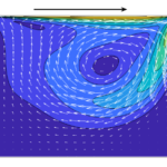
This lid-driven cavity flow calculator converts cavity size, lid speed and kinematic viscosity into the Reynolds number, Re = UL/ν. It then computes a steady two-dimensional flow field, estimates the primary vortex position and plots the horizontal and vertical centreline velocities. All coordinates in the drawing are divided by the cavity side length. The origin is the bottom left corner, the lid moves to the right, and positive vertical velocity points upward.
Enter the fluid viscosity at the temperature of interest, the internal side length and the lid speed. The initial example uses a 0.1 m cavity, a 0.001 m/s lid and ν = 1 mm²/s (10⁻⁶ m²/s), giving Re = 100. The metric/US control converts the dimensional entries and position results. To reproduce Re = 400 with the other defaults, set the lid speed to 0.004 m/s.
Fast mode solves 25×25 nodes and compares them with 13×13 nodes. Refinement mode solves 33×33 nodes and compares them with 17×17 nodes; it takes longer. Both use fourth-order interior differences, a compact streamfunction Poisson equation and a banded modified Newton iteration for steady vorticity transport. The converged coarse field initializes the fine solve, and mesh-only operators are cached. These are independent numerical implementations of the equations discussed in the linked WiredWhite articles. They do not reproduce the articles’ RK2/SOR startup simulation.
Read the convergence results before using the vortex coordinates. The transport residual measures how closely the discrete steady equations balance. The two-grid change is the largest difference between either centreline velocity profile at common grid stations, divided by lid speed. The default screening targets are a residual below 10⁻⁶ and a profile change below 3% of lid speed. Meeting both targets is useful evidence, but two meshes do not establish an observed order, a Grid Convergence Index or a rigorous error bound. The comparison table also shows the movement of the primary vortex.
Press play to follow tracers through the computed, frozen velocity field. Tracer time is tU/L; tracers restart after 30 units. This animation illustrates circulation, not the physical startup from rest.
Use this tool for laminar square-cavity studies over 1 ≤ Re ≤ 1000. Corner singularities, small secondary vortices and high-Reynolds-number shear layers need finer external CFD meshes. The calculator does not predict three-dimensional instabilities, turbulence, pressure, wall forces, heat transfer, free surfaces or non-Newtonian behaviour. Benchmark checks use published Ghia vortex positions and centreline velocity extrema at Re = 100 and 400, with explicit tolerances appropriate to these small grids.
How it is calculated
The length and velocity scales are and , giving . The coordinates start at the bottom left; the lid moves right. Define , and . The steady equations are
These are the equations discussed in WiredWhite post 39865. Post 45218 describes a different, pressure-projection solution of the same cavity problem.
The implementation here is derived from these equations. Uniform grids use fourth-order centred first and second derivatives, with fourth-order one-sided derivatives at the first interior line. A nine-point compact Poisson stencil satisfies . At a stationary wall the one-sided vorticity closure is ; the moving top adds . These coefficients follow from Taylor expansion, not benchmark fitting. The lid corners are assigned the stationary-wall velocity.
Keep streamfunction and scaled vorticity as coupled unknowns. Group them by grid row and factor the nonzero bands of the analytic Jacobian. The largest dense pivot is 62×62, rather than a full-grid dense system. Mesh-only derivative matrices and the coarse-grid Stokes estimate are cached separately. The coarse solve uses Reynolds-number continuation with increments no larger than 600. Bilinear prolongation of its converged streamfunction and vorticity initializes the fine solve at the requested Re.
A damped modified Newton iteration reuses a factorization while the residual contracts by at least a factor of 0.4; otherwise it rebuilds the Jacobian. A halving line search reduces the transport imbalance. Each stage stops below a maximum dimensionless transport residual of or after 40 updates. The reported residual is evaluated from the final fields, including when the iteration limit is reached. The compact Poisson residual and discrete divergence are evaluated separately. This is a steady solver, not an RK2/SOR transient reproduction.
The primary vortex is the most negative streamfunction node, refined by a local two-dimensional quadratic. Both velocity minima are sampled on the complete centreline, including the walls. Compare both grid profiles at common nodes: . The screening targets are on both grids and . A small residual does not measure discretization error. Tracers use midpoint integration and bilinear sampling of a cached velocity field; their positions alone change during play.
Assumptions
Steady, two-dimensional, incompressible Newtonian flow; constant kinematic viscosity; a square cavity; a uniform rightward lid speed; three stationary no-slip walls; no body forces. All solver variables are dimensionless. The finite-difference equations and wall coefficients are derived here. No empirical vortex-position correlation or benchmark table is used in the solver. The two-grid comparison uses identical discretization methods. The tracer animation is a visualization of the frozen field and restarts after 30 units of tU/L.
Where it applies
Use over 1 ≤ Re ≤ 1000. Fast mode uses 13×13 and 25×25 nodes; refinement mode uses 17×17 and 33×33. Browser cost rises with mesh size and Reynolds number. Both mesh options are screened across the supported range; the tracer animation reuses cached fields. The Re = 100 and 400 checks accept finite-grid differences explicitly: up to 0.01–0.02 L in vortex coordinates and 0.007–0.025 U in the centreline minima. These tolerances are test criteria, not confidence intervals. Above Re = 400 the small grids can significantly under-resolve wall shear and corner vortices. The lid/wall velocity discontinuity makes global formal order uncertain. Two grids cannot establish an observed order, GCI or rigorous error bound; the grid-change target concerns centreline velocities only. This tool does not calculate pressure, forces, turbulence, three-dimensional instability, heat transfer or actual startup time. No symmetry of the lid-driven velocity profiles is assumed. Smooth contours alone do not validate a solution.
References
- Waqas Javaid, High-Resolution CFD Analysis of Incompressible Flow in a Lid-Driven Cavity Using Explicit RK2 and SOR Techniques, WiredWhite, post 39865: https://wiredwhite.com/cfd-lid-driven-cavity-rk2-sor-matlab/
- WiredWhite, Numerical Exploration of Vortex Dynamics, Solving the Incompressible Navier-Stokes Equations Using Matlab, post 45218: https://wiredwhite.com/vortex-dynamics-navier-stokes-matlab/
- U. Ghia, K. N. Ghia and C. T. Shin (1982), High-Re solutions for incompressible flow using the Navier-Stokes equations and a multigrid method, Journal of Computational Physics 48, 387–411. DOI: https://doi.org/10.1016/0021-9991(82)90058-4. Tables I–II: centreline velocities; Table III: vortex properties.
- B. J. Smith et al. (2024), Laminar boundary layer separation and reattachment on a rotating sphere, Appendix B and Table 2 (PDF p. 22 reproduce Ghia vortex centres). DOI: https://doi.org/10.1017/jfm.2024.173.
- J.-P. Wang, J.-F. Zhang, Z.-G. Qu and W.-Q. Tao (2020), An adaptive inner iterative pressure-based algorithm for steady and unsteady incompressible flows, Table III: independent CFD comparison reproducing Ghia velocity extrema. DOI: https://doi.org/10.1108/HFF-09-2018-0483. Author-hosted copy: https://nht.xjtu.edu.cn/202020E.pdf
Inputs
| Input | Symbol | Unit | Default |
|---|---|---|---|
| Cavity side length Internal side length of the square cavity. | L_c | m | 0.1 |
| Lid speed to the right Positive horizontal speed of the top wall; the other walls are stationary. | U_lid | m/s | 0.001 |
| Kinematic viscosity Enter kinematic viscosity in mm²/s (1 mm²/s = 10⁻⁶ m²/s). Use the value at the operating temperature. | nu_k | mm^2/s | 1 |
| Grid pair Refinement mode costs more time. Each pair uses the same equations and boundary conditions. | mesh | Fast: 13×13 and 25×25 nodes | |
| Tracer time, tU/L Play follows the frozen flow field. It does not advance the CFD solution or simulate startup. | t_star | 6 |
Results
With the default inputs above, the calc gives:
| Result | Value |
|---|---|
| Reynolds number | 100 |
| Vortex x from left wall | 0.0613 m |
| Vortex y above bottom | 0.0737 m |
| Centreline minimum u/U | -0.2134 |
| Centreline minimum v/U | -0.2488 |
| Two-grid change (% of lid speed) | 2.132 |
| Steady transport residual | 4.72e-7 |
| Convergence assessment | Residual and two-grid targets met |
Checked against sources
Each case below was calculated by this calc and agrees with the value from its source (within the tolerance where one is shown).
Ghia Re = 100 · vortex and both centreline minima
Source: Ghia, Ghia and Shin (1982), DOI 10.1016/0021-9991(82)90058-4, Tables I–III. Primary centre (0.6172, 0.7344), u/U minimum −0.21090 at y/L = 0.4531, v/U minimum −0.24533 at x/L = 0.8047. Vortex data reproduced in Smith et al. (2024), DOI 10.1017/jfm.2024.173, Table 2, attached PDF p. 22. Velocity extrema independently reproduced by Wang et al. (2020), Table III, DOI 10.1108/HFF-09-2018-0483, https://nht.xjtu.edu.cn/202020E.pdf. Absolute acceptance tolerances allow the finite 25×25 grid; they are not fitted corrections or error bounds.
Inputs: the default inputs above.
| Result | Source | This calc |
|---|---|---|
| Reynolds number | 100 | 100 |
| Primary vortex x/L | 0.6172 ± 0.01 | 0.6127 |
| Primary vortex y/L | 0.7344 ± 0.01 | 0.7374 |
| Centreline minimum u/U | -0.2109 ± 0.007 | -0.2134 |
| Centreline minimum v/U | -0.2453 ± 0.009 | -0.2488 |
| Minimum dimensionless streamfunction | -0.1034 ± 0.002 | -0.1031 |
Ghia Re = 400 · refined grid, vortex and velocity minima
Source: Ghia, Ghia and Shin (1982), DOI 10.1016/0021-9991(82)90058-4, Tables I–III. Primary centre (0.5547, 0.6055), u/U minimum −0.32726 at y/L = 0.2813, v/U minimum −0.44993 at x/L = 0.8594. Smith et al. (2024), DOI 10.1017/jfm.2024.173, attached PDF p. 22, Table 2 reproduces vortex data and flags an anomalous Ghia v(x,0.5) point near x = 0.9. That outlying point is not used as the minimum. Velocity extrema are independently reproduced in Wang et al. (2020), DOI 10.1108/HFF-09-2018-0483, Table III, https://nht.xjtu.edu.cn/202020E.pdf. The 33×33-grid velocity acceptance bands are 0.012 U and 0.025 U; residual convergence is assessed separately and no formula is adjusted to the benchmark.
Inputs: Lid speed to the right = 0.004 m/s; Grid pair = Refine: 17×17 and 33×33 nodes; the others as above.
| Result | Source | This calc |
|---|---|---|
| Reynolds number | 400 | 400 |
| Primary vortex x/L | 0.5547 ± 0.01 | 0.5551 |
| Primary vortex y/L | 0.6055 ± 0.02 | 0.6102 |
| Centreline minimum u/U | -0.3273 ± 0.012 | -0.32 |
| Centreline minimum v/U | -0.4499 ± 0.025 | -0.4325 |
| Minimum dimensionless streamfunction | -0.1139 ± 0.004 | -0.1117 |









Responses