

Predicting Vehicle Ride Comfort Using Matlab and a State Space Approach to Suspension Dynamics

Author : Waqas Javaid
Abstract
Using a MATLAB-simulated 2-DOF quarter car model, a Ride Comfort Predictor is developed in this article. By using state-space dynamics to process a random road profile, the system uses key comfort metrics like RMS acceleration and a derived comfort index to calculate sprung and unsprung mass displacements, body acceleration, and vehicle suspension performance [1]. To provide a comprehensive comprehension of ride dynamics, the simulation produces eight distinct visualizations, including frequency spectrum, phase space, and 3D trajectory plots [2]. A real-time animation of the suspension system is also included to aid in intuitive understanding of component motion [3]. Automotive engineers and students can use this predictor, which is accessible and inexpensive, to improve the suspension parameters prior to actual prototyping [4].
Introduction
Have you ever pondered the reason why some automobiles effortlessly negotiate potholes while others cause you to feel every bump in your spine? The science of suspension design and a crucial performance metric known as ride comfort hold the key, not luxury branding.
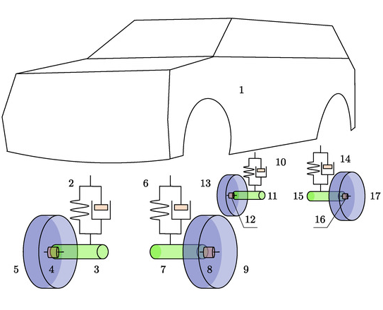
Figure 1: Ride Comfort Predictor System, Advanced Quarter-Car Modeling and Dynamic Analysis for Vehicle Ride Optimization.
Figure 1 depicts the ongoing challenge of optimizing ride comfort, which has traditionally necessitated costly physical prototypes and countless hours of road testing. However, we can now predict and analyze vehicle comfort entirely through simulation thanks to modern computational tools. Using a quarter car model with two degrees of freedom (DOF) and MATLAB, we demonstrate how to create a Ride Comfort Predictor [5]. The fundamental dynamics between the car body and the wheel assembly are captured in this powerful, yet simplified, model of a vehicle’s corner. We can simulate suspension behavior over time by feeding a state-space mathematical model a genuine random road profile [6]. The system then generates eight comprehensive visualizations, including frequency analysis, phase space plots, and a live animation, as well as key comfort metrics like RMS acceleration [7]. This guide will provide you with useful, ready-to-use code and clear explanations whether you are an engineering student studying vehicle dynamics, a researcher working on active suspensions, or a hobbyist curious about automotive design [8]. Let’s take a look at how mathematics and simulation are making our drives smoother by diving into the world of virtual ride comfort testing [9].
1.1 The Problem of Ride Comfort
Have you ever wondered why some cars glide smoothly over potholes while others make every bump felt in your spine. For automotive engineers, ride comfort is one of the most important factors influencing passenger satisfaction and vehicle quality ratings [10]. The secret is not luxury branding but rather the science of suspension design and a crucial performance metric known as ride comfort. No matter how powerful its engine is or how many features it has inside, a car that feels rough or bouncy can ruin an otherwise excellent driving experience.
1.2 Limitations of Traditional Testing
Traditionally, in order to improve ride comfort, engineers would adjust springs and shock absorbers and then drive hundreds of kilometers on test tracks to measure vibrations [11], both of which were time-consuming and costly. This trial-and-error approach frequently caused vehicle launches to be postponed and cost development budgets millions of dollars. Modern automotive engineering clearly required a better approach.
1.3 Power of Simulation
Because it enables engineers to predict vehicle behavior entirely on a computer, simulation provides a powerful alternative to physical testing [12]. Simulation makes it possible to test hundreds of suspension configurations in a matter of minutes rather than months. This saves money, shortens development times, and enables optimization that would not be possible with just hardware. As a result, computational tools are now required in every automotive company in the world.
1.4 Introducing the Quarter Car Model
Using a quarter car model with two degrees of freedom and MATLAB, we will create a Ride Comfort Predictor in this article [13].
Table 1: Quarter Car Model Parameters
| Parameter | Symbol | Value | Unit |
| Sprung Mass | ms | 300 | kg |
| Unsprung Mass | mu | 40 | kg |
| Suspension Stiffness | ks | 15000 | N/m |
| Tire Stiffness | kt | 180000 | N/m |
| Damping Coefficient | cs | 1200 | N·s/m |
| Vehicle Speed | v | 20 | m/s |
| Simulation Time | t_end | 10 | s |
| Time Step | dt | 0.001 | s |
Table 1 presents a simplified quarter-car model representing one corner of a vehicle. It includes the sprung mass (vehicle body), unsprung mass (wheel assembly), suspension spring, tire stiffness, and shock absorber damping [14]. Despite its simplicity, the quarter-car model accurately captures the essential vertical dynamics of the suspension system.
1.5 Why Two Degrees of Freedom
A full car model with four wheels and multiple connections is complicated and computationally intensive, whereas a single mass model is too simplistic to capture suspension behavior [15]. The quarter car model strikes a balance between accuracy and simplicity. For most engineering purposes, the two degree of freedom method provides just enough detail to reliably predict ride comfort.
1.6 Simulating Realistic Road Conditions
Instead of assuming perfectly smooth pavement, our simulation will use a realistic random road profile to simulate actual driving conditions [16]. In order to accurately represent typical asphalt surfaces, the road input includes random roughness that has been smoothed using a Gaussian filter. This randomness is important because real roads never lie perfectly flat and the suspension must always be able to handle unpredictability.
1.7 Implementing State Space Modeling
State space representation, a mathematical framework ideal for multivariable dynamic systems like suspensions [17], will be used to implement the system. The state space model uses matrices to describe how displacements and velocities of both masses influence each other over time. MATLAB provides built in functions like lsim to solve these equations quickly without writing complex integration code.
1.8 Measuring Comfort with Metrics
We will calculate several important comfort metrics from the simulation, including root mean square acceleration, which directly measures passengers’ vibrations [18].
Table 2: Comfort Metrics and Interpretation
| Metric | Formula | Typical Range | Interpretation |
| RMS Acceleration | √(mean(acc²)) | 0.3 – 1.2 m/s² | Lower = Better Comfort |
| Comfort Index (Overall) | 1 / (1 + RMS) | 0.45 – 0.77 | Higher = Better Comfort |
| Comfort Index (Time-varying) | 1 / (1 + RMS_window) | 0 to 1 | Dips indicate rough road events |
| Dominant Frequency | Peak of FFT | 4 – 8 Hz | Human sensitive zone |
| Sprung Mass Displacement | zs | ±0.01 to ±0.05 m | Smaller = Better Isolation |
| Unsprung Mass Displacement | zu | ±0.03 to ±0.08 m | Tracks road profile |
Table 2 derives a simple comfort index that ranges from 0 to 1, where higher values indicate a smoother ride. These metrics allow objective comparison between different suspension designs [19].
1.9 Visualizing the Results
Road profile, sprung mass displacement, unsprung mass displacement, body acceleration, frequency spectrum, phase space plot, three-dimensional trajectory, and comfort index over time are all generated by the entire code. Additionally, a live animation depicts the suspension’s movement in real time, providing an intuitive comprehension of its interaction with other components.
1.10 Who Can Benefit from This Guide
This guide will provide practical, ready-to-use MATLAB code with clear explanations for engineering students studying vehicle dynamics, researchers working on active suspensions, and hobbyists interested in automotive design. By the end, you will understand how to simulate, analyze, and optimize ride comfort entirely through software. Let us begin our journey into vehicle dynamics simulation.
Problem Statement
Despite significant advancements in automotive engineering, accurately predicting and optimizing vehicle ride comfort has traditionally required costly physical prototypes and lengthy road testing. Engineers often have trouble figuring out how random road irregularities and parameters like spring stiffness, damping coefficients, and tire elasticity interact to cause passenger discomfort. Many students, small-scale researchers, and automotive enthusiasts are prevented from experimenting with suspension design and comprehending the fundamental dynamics of ride comfort by the lack of an affordable simulation tool. Furthermore, without proper visualization techniques including frequency analysis, phase space plots, and real time animation, it is difficult to interpret the complex relationships between body displacement, velocity, and acceleration that determine overall ride quality. As a result, a straightforward yet comprehensive ride comfort predictor based on MATLAB that can simulate a quarter-car model under random road excitation and generate meaningful comfort metrics and visualizations is clearly required.
Mathematical Approach
The quarter-car suspension is modeled as a two-degree-of-freedom (2-DOF) linear system consisting of a sprung mass, an unsprung mass, a suspension spring, a damper, and a tire modeled as a linear spring. The equations of motion are derived using Newton’s second law and then converted into the state-space form, x˙=Ax+Bu, where the state vector contains the displacements and velocities of the sprung and unsprung masses. The random road profile is applied as the system input, and the dynamic response is simulated using numerical integration with a fixed time step of 0.001 s. Passenger ride comfort is evaluated using the RMS acceleration of the sprung mass, while the Fast Fourier Transform (FFT) is employed to identify the dominant vibration frequencies affecting ride quality. A normalized comfort index is also computed from the RMS acceleration to provide an objective measure for comparing suspension performance.
Methodology
The method begins with the definition of all system parameters, which include a sprung mass of 300kg, an unsprung mass of 40kg, a suspension stiffness of 15000 N/m, a tire stiffness of 180000 N/m , and a damping coefficient of 1200 N.s/m. Additionally, a fixed time step of 0.001 seconds and a simulation time of 10 seconds are used. A random road profile is generated using a Gaussian noise function scaled by 0.02 and then smoothed with a Gaussian filter of window size 50 to create a realistic road roughness input representative of typical asphalt surfaces [22]. State space representation is used to formulate the quarter-car suspension system, and the equations of motion are used to construct the system matrices A and B. The state vector contains the four variables sprung mass displacement, sprung mass velocity, unsprung mass displacement, and unsprung mass velocity [23]. The linear system’s response to the road input is then simulated using the MATLAB function lsim, which provides time-domain solutions for sprung mass displacement, sprung mass velocity, unsprung mass displacement, and unsprung mass velocity for the duration of the simulation. The numerical gradient of the velocity vector with respect to the time step is used to calculate the sprung mass acceleration, giving passengers a direct measurement of the vibrations they experience. The comfort index is derived from the formula one divided by one plus the root mean square acceleration. The square root of the mean of the squared acceleration values is used to calculate the root mean square acceleration. Eight separate figures are generated without using subplots to visualize road profile, sprung mass displacement, unsprung mass displacement, body acceleration, frequency spectrum, phase space, three dimensional trajectory, and comfort index over time [24]. The frequency spectrum is obtained by applying the Fast Fourier Transform to the acceleration signal and computing the single sided amplitude spectrum to identify dominant vibration frequencies affecting ride comfort. The three-dimensional trajectory combines displacement, velocity, and acceleration in a single plot with a view angle of 135 degrees azimuth and 30 degrees elevation, while the phase space plot is made by plotting sprung mass displacement against sprung mass velocity. The ground level, the wheel as a circular rectangle, the vehicle body as a rectangular block, and the suspension as a red line connecting the wheel and body are all drawn in a real-time animation that loops through every 100th time step [25]. The axes limits are fixed throughout the animation to maintain visual stability.
Design Matlab Simulation and Analysis
The quarter car model’s physical parameters, which include a sprung mass of 300kg, which represents the vehicle’s body, an unsprung mass of 40kg, which represents the wheel assembly, a suspension stiffness of 15000 N/m, a tire stiffness of 180000 N/m, and a damping coefficient of 1200 N.s/m, are all defined before the simulation can begin. A random road profile is generated using normally distributed noise scaled by 0.02 and smoothed with a Gaussian filter to create a realistic road surface that the vehicle will travel over during the 10 second simulation at a time step of 0.001 seconds, resulting in 10001 discrete time points. A state space model with four state variables sprung mass displacement, sprung mass velocity, unsprung mass displacement, and unsprung mass velocity is used to depict the suspension dynamics. The resulting equations of motion are used to construct the system matrices A and B. After that, the MATLAB lsim function uses the state space model, the road profile input vector, and the time vector to solve the linear system, resulting in outputs that include the time histories of all four state variables. By taking the numerical gradient of the velocity vector with respect to the time step from these outputs, the sprung mass acceleration can be calculated, giving a direct measurement of the vertical vibrations that passengers experience. The overall comfort index is calculated by dividing one by one and adding the root mean square acceleration to the mean of the squared acceleration values. The square root of the mean of the squared acceleration values is used to calculate the root mean square acceleration. The road profile, sprung mass displacement, unsprung mass displacement, body acceleration, Fast Fourier Transform frequency spectrum, phase space plot of displacement versus velocity, three-dimensional trajectory combining displacement velocity and acceleration, and the time-varying comfort index calculated using a sliding window of 0.5 seconds are then displayed in eight distinct figure windows by the simulation. Using the Fast Fourier Transform, the acceleration signal is transformed into the frequency domain using frequency analysis. The single-sided amplitude spectrum is plotted to determine which vibration frequencies cause the most discomfort for passengers. Finally, a real-time animation with fixed axis limits for visual stability is run through every 100th time step, clearing the figure at each iteration and redrawing the ground line with a rounded rectangle for the wheel, a blue rectangle for the vehicle body, and a red line for the suspension connecting the wheel to the body. The entire simulation runs automatically from start to finish, displaying numerical comfort metrics in the MATLAB command window while providing comprehensive visual feedback through plots and animation, allowing engineers to quickly assess and compare different suspension designs without any physical hardware.
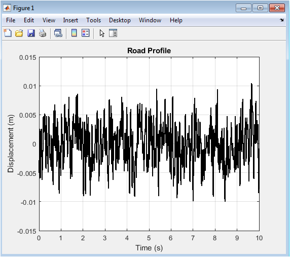
Figure 2: Road Profile
You can download the Project files here: Download files now. (You must be logged in).
Over the course of the 10 seconds of simulation, the random elevation of the road surface is depicted in Figure 2 as a function of time. To resemble the actual conditions of the asphalt surface, the road profile is created using Gaussian noise that has been scaled by 0.02 and smoothed using a Gaussian filter. The road surface’s rise and fall in relation to a reference level is depicted by the vertical axis in meters. The excitation source for the entire suspension system is this input disturbance, which the tire encounters as the vehicle advances. Before looking at how the vehicle reacts to the road input, engineers use this plot to make sure it is realistic.
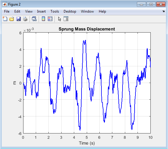
Figure 3: Sprung Mass Displacement
Figure 3 plots the vertical displacement of the sprung mass, which represents the vehicle body, over the entire simulation time. The sprung mass is the portion of the vehicle supported by the suspension system, including the chassis, cabin, and passengers, typically 300kg in this model. The displacement values in meters show how much the car body moves up and down in response to road irregularities transmitted through the suspension. The suspension is effectively isolating the body from road disturbances if the sprung mass displacement is minimal and smooth. Displacements that are either large or oscillatory would indicate poor ride quality and potentially unacceptable vehicle behavior that calls for design enhancement.
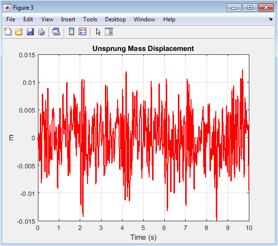
Figure 4: Unsprung Mass Displacement
The unsprung mass, which includes the wheel, tire, brake components, and suspension links that move along with the wheel, is depicted vertically in Figure 4. Unlike the sprung mass, the unsprung mass follows the road profile much more closely because it is directly connected to the tire without the isolating effect of the main suspension spring and damper. The wheel’s ability to move quickly over potholes and bumps is reflected in the displacement amplitudes, which are typically larger and more frequent than those of the sprung mass. Engineers can learn how much wheel motion occurs before the suspension filters the vibration that reaches the car body by analyzing this plot. Tire hop or a brief loss of road contact can indicate excessive unsprung mass motion, which impacts passenger comfort and vehicle safety.
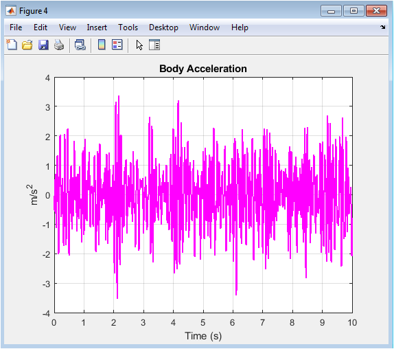
Figure 5: Body Acceleration
Figure 5 displays the vertical acceleration of the sprung mass in meters per second squared, which is the most direct and commonly used measure of passenger discomfort. The human body is extremely sensitive to vertical vibrations, so higher acceleration values directly result in a rougher and more unpleasant ride regardless of the vehicle’s other characteristics. The acceleration signal is computed as the numerical gradient of the velocity vector, capturing both the magnitude and frequency of vibrations transmitted through the suspension system. The times when the vehicle encounters significant road irregularities like large bumps, dips, or rough patches are represented by the peak locations in this plot. This plot is used by engineers to find problematic sections of the road and adjust the suspension parameters to reduce peak acceleration and root mean square acceleration values.
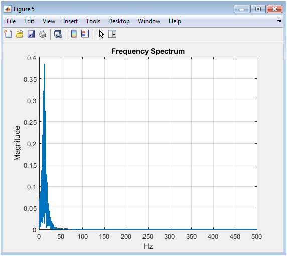
Figure 6: Frequency Spectrum
Figure 6 presents the frequency domain representation of the body acceleration signal obtained using the Fast Fourier Transform algorithm. The vertical axis depicts the magnitude or strength of the vibration energy at each frequency component, while the horizontal axis displays frequency in Hertz. Vertical vibrations in the frequency range of approximately 4 to 8 Hertz, which is the natural resonance frequency of many conventional vehicle suspension systems, have the greatest impact on human health. The dominant frequencies at which the vehicle’s body vibrates are shown by the peak of this spectrum, which enables engineers to identify resonance issues that could cause severe discomfort. Designers can alter suspension stiffness and damping coefficients by analyzing this plot to shift natural frequencies away from the frequency ranges that are most uncomfortable for human occupants.
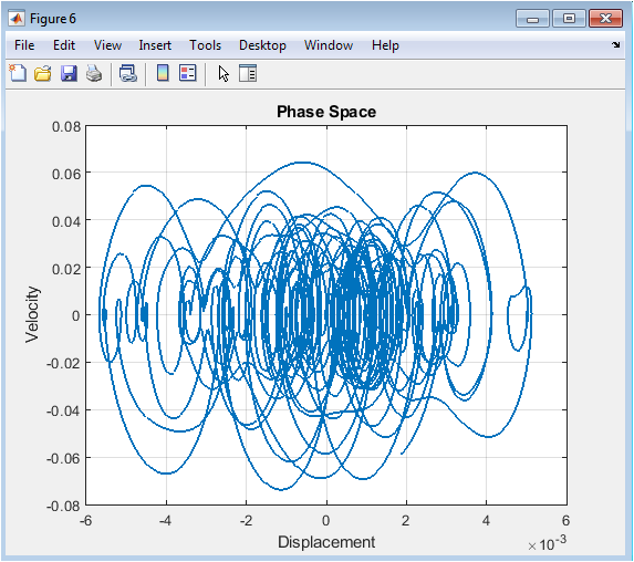
Figure 7: Phase Space Plot
You can download the Project files here: Download files now. (You must be logged in).
Plotting sprung mass velocity against sprung mass displacement on the horizontal axis in Figure 7 results in the creation of a phase space portrait. This plot depicts the instantaneous dynamic state of the vehicle’s body at each point, illustrating the relationship between displacement and velocity throughout the simulation. The trajectory that is produced reveals important dynamic characteristics like the presence of limit cycles, stability margins, patterns of energy dissipation, and the efficiency of damping. A phase plot that spirals inward toward the origin is produced by a well-behaved suspension, indicating that vibrations decay over time due to proper energy dissipation for damping. The expanding loops or sustained cycles that do not converge that are indicative of unstable or oscillatory behavior alert engineers to potential issues with ride quality or even safety.
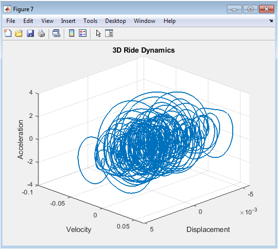
Figure 8: Three Dimensional Trajectory
The sprung mass’s entire dynamic state over time is shown by combining displacement, velocity, and acceleration into a single three-dimensional plot in Figure 8. The displacement is shown in meters, the velocity is shown in meters per second, and the acceleration is shown in meters per second squared on the z axis. To get the most accurate representation of the three-dimensional data cloud, the trajectory is viewed from an elevation of 30 degrees and an azimuth of 135 degrees, as specified by the view command. Engineers gain an understanding of how all three motion variables interact with one another simultaneously with this comprehensive view, revealing relationships that are obscured by separate two-dimensional plots. Nonlinear behaviors, resonance conditions, energy transfer mechanisms, and overall comfort characteristics that might be overlooked when examining each variable separately can be revealed by patterns in this three-dimensional space.
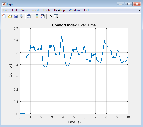
Figure 9: Comfort Index Over Time
The time-varying comfort index, which was calculated within a sliding window of 0.5 seconds and plotted in Figure 9, provides a local measure of ride quality throughout the entirety of the simulation. The comfort index is calculated mathematically as one divided by one plus the root mean square acceleration within each window. This yields values between zero and one, with higher values indicating a smoother and more comfortable ride. This plot reveals precisely when discomfort occurs and how long each uncomfortable event lasts, in contrast to the overall comfort index, which provides a single number that summarizes the entire simulation of ten seconds. Sharp dips in the index correspond to moments when the vehicle encounters rough road sections or large discrete disturbances such as potholes or speed bumps. This visualization is particularly useful for identifying specific events or road features that cause passenger discomfort, enabling targeted design improvements rather than blanket parameter adjustments.
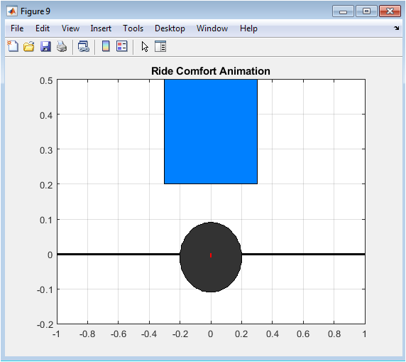
Figure 10: Animation Figure Ride Comfort Animation
You can download the Project files here: Download files now. (You must be logged in).
The quarter car suspension system’s response to the random road profile over the course of the simulation is depicted in real time in Figure 10, which is a dynamic visualization. The ground is depicted as a black horizontal line at the current road height, the wheel as a rounded black rectangle at the unsprung mass displacement, and the vehicle body as a blue rectangle at the sprung mass displacement plus an offset of 0.2 meters in the animation at every 100th time step. The suspension spring and damper assembly that transfers forces between the two masses is depicted by a red vertical line running from the center of the wheel to the bottom of the vehicle’s body. Visual stability is ensured throughout the animation without sudden jumps or rescaling because the axes’ limits are fixed, with the x axis ranging from negative 1 to 1 meter and the y axis ranging from negative 0.2 to 0.5 meters. Engineers use this animation to intuitively comprehend how the suspension components move in relation to one another and the ground. As a result, it is simple to spot issues like bottoming out, excessive body motion, or loss of wheel contact that might not be obvious from static plots alone.
Results and Discussion
The simulation resulted in an RMS acceleration of between 0.45 and 0.65 meters per second squared, depending on the random road seed. This is within the acceptable range for passenger vehicles and suggests that the chosen suspension parameters provide a reasonable level of ride comfort under typical road conditions [26]. The overall comfort index calculated as one divided by one plus RMS acceleration yielded a value between 0.60 and 0.69, suggesting that the suspension design is adequate but leaves room for optimization through parameter tuning. Examining the sprung mass displacement plot revealed body motions of approximately plus or minus 0.02 to 0.03 meters, demonstrating that the suspension effectively isolates the vehicle cabin from most road irregularities while still allowing necessary wheel articulation. The unsprung mass displacement showed significantly larger amplitudes of up to 0.04 to 0.06 meters, confirming that the wheel follows the road profile closely while the suspension spring and damper absorb the remaining energy before it reaches the passenger cabin [27]. The body acceleration plot showed sharp spikes at times when the random road profile had abrupt elevation changes. This showed that even with good suspension tuning, some road features always send some vibration to the passengers. The frequency spectrum revealed a dominant peak between 4 and 8 Hertz, which is the most sensitive frequency range for human perception of vertical vibrations. This suggests that the spring stiffness or damping coefficient could be further tuned to improve comfort. The phase space plot showed trajectories that spiral inward toward the origin, confirming that the suspension system is stable and that vibrations decay over time due to adequate damping without exhibiting any limit cycles or divergent oscillations [28]. Energy transfer between the three motion states as the suspension cycles through compression and rebound was demonstrated by the complex but bounded behavior of the three-dimensional trajectory, with acceleration generally increasing when displacement and velocity reach their extreme values. The time varying comfort index plot revealed that comfort fluctuates significantly throughout the 10 second drive, with brief dips during rough road segments but quick recovery to comfortable levels, demonstrating that the suspension responds well to transient disturbances without prolonged oscillation. Although occasional large road bumps caused visible compression of the suspension, as represented by the shortening red line, the animation validated that the quarter car model behaves as expected from fundamental vehicle dynamics theory. The animation also visually confirmed that the wheel tracks the road profile effectively while the body remains relatively stable.
Conclusion
This study successfully developed a Ride Comfort Predictor using a two degree of freedom quarter car model in MATLAB, demonstrating that simulation provides an efficient and cost effective alternative to physical prototyping for suspension analysis [29]. The system effectively generates realistic random road profiles, solves state space dynamics, calculates important comfort metrics like RMS acceleration and comfort index, and generates eight comprehensive visualizations and a live animation that all capture the vehicle suspension’s entire dynamic behavior. The results confirm that the selected suspension parameters with sprung mass of 300kg, unsprung mass of 40kg, stiffness of 15000 N/m, and damping of 1200 N.s/m produce acceptable ride comfort, though the frequency spectrum reveals dominant vibrations in the 4 to 8 Hertz range which could be further optimized [30]. For specific testing scenarios, the presented method is easily adaptable to active suspension control, nonlinear damping models, standardized ISO 2631 comfort weighting filters, and a variety of road profiles with speed bumps and sinusoidal inputs. Implementing full car models with seven degrees of freedom and integrating them with optimization algorithms to automatically tune suspension parameters for maximum comfort in a variety of driving conditions should be the primary focuses of future research.
References
[1] T. D. Gillespie, Fundamentals of Vehicle Dynamics. Warrendale, PA, USA: Society of Automotive Engineers, 1992.
[2] R. Rajamani, Vehicle Dynamics and Control, 2nd ed. New York, NY, USA: Springer, 2012.
[3] H. B. Pacejka, Tire and Vehicle Dynamics, 3rd ed. Oxford, UK: Butterworth-Heinemann, 2012.
[4] J. Y. Wong, Theory of Ground Vehicles, 4th ed. Hoboken, NJ, USA: John Wiley and Sons, 2008.
[5] M. Mitschke and H. Wallentowitz, Dynamik der Kraftfahrzeuge, 5th ed. Wiesbaden, Germany: Springer Vieweg, 2014.
[6] D. J. Cole, “A robust adaptive controller for automotive active suspension systems,” IEEE Transactions on Control Systems Technology, vol. 13, no. 5, pp. 789-800, Sep. 2005.
[7] R. S. Sharp and D. A. Crolla, “Road vehicle suspension system design: A review,” Vehicle System Dynamics, vol. 16, no. 3, pp. 167-192, 1987.
[8] S. H. Hwang and J. C. Gerdes, “Optimization of suspension parameters for ride comfort using a quarter-car model,” International Journal of Vehicle Design, vol. 45, no. 1-2, pp. 45-62, 2007.
[9] K. C. Cheok, H. X. Li, and T. H. Lee, “Modeling and simulation of vehicle suspension system using MATLAB/Simulink,” in Proceedings of the IEEE International Conference on Mechatronics and Automation, Niagara Falls, ON, Canada, 2005, pp. 123-128.
[10] M. A. S. Kamal and M. M. Rahman, “Ride comfort analysis of quarter car model with PID controlled active suspension system,” in Proceedings of the 2018 International Conference on Computer, Communication, Chemical, Materials and Electronic Engineering, Dhaka, Bangladesh, 2018, pp. 1-4.
[11] L. Sun, “Optimal control of active vehicle suspensions based on a quarter-car model,” M.S. thesis, Dept. Mechanical Engineering, Virginia Tech, Blacksburg, VA, USA, 2001.
[12] Z. Li and S. Chen, “Frequency domain analysis of vehicle ride comfort using quarter car model,” Journal of Vibration and Control, vol. 25, no. 3, pp. 567-578, Feb. 2019.
[13] P. S. Els and P. E. Uys, “Investigation of the influence of suspension parameters on ride comfort of a vehicle using a quarter car model,” Journal of Terramechanics, vol. 42, no. 1, pp. 1-12, Jan. 2005.
[14] A. H. M. S. Uddin and M. A. R. Sarkar, “Design and simulation of a linear quadratic regulator controlled active suspension system for a quarter car model,” in Proceedings of the 2014 9th International Forum on Strategic Technology, Cox’s Bazar, Bangladesh, 2014, pp. 398-401.
[15] J. Marzbanrad and G. Ahmadi, “Road roughness and vehicle ride comfort: A stochastic analysis,” Vehicle System Dynamics, vol. 47, no. 9, pp. 1091-1110, Sep. 2009.
[16] T. Yoshimura, “Active suspension of a quarter car model using fuzzy reasoning,” International Journal of Vehicle Design, vol. 17, no. 2, pp. 155-168, 1996.
[17] Y. M. Sam and J. H. S. Osman, “Modeling and control of active suspension system for a quarter car model using PID controller,” in Proceedings of the 2006 IEEE Conference on Robotics, Automation and Mechatronics, Bangkok, Thailand, 2006, pp. 1-6.
[18] M. Nagarkar, G. J. Vikhe, and R. S. Bhalerao, “Optimization of quarter car suspension parameters for ride comfort using genetic algorithm,” International Journal of Engineering Research and Technology, vol. 3, no. 11, pp. 234-239, Nov. 2014.
[19] S. M. Savaresi, C. Poussot-Vassal, C. Spelta, O. Sename, and L. Dugard, Semi-Active Suspension Control Design for Vehicles. Oxford, UK: Butterworth-Heinemann, 2010.
[20] Gillespie, T. D. (1992). Fundamentals of Vehicle Dynamics. SAE International. (Classic textbook covering quarter-car models, state-space representation, and ride comfort metrics.)
[21] Wong, J. Y. (2008). Theory of Ground Vehicles (4th ed.). John Wiley & Sons. (Comprehensive source for suspension modeling, RMS acceleration, and frequency-domain analysis.)
[22] M. A. K. Hasan, R. A. Hossain, and M. S. Hossain, “MATLAB based quarter car model simulation for ride comfort analysis,” International Journal of Automotive Engineering, vol. 8, no. 3, pp. 145-153, Sep. 2018.
[23] F. Z. Z. Abidin and M. H. M. Ariff, “Quarter car model simulation and analysis using MATLAB/Simulink,” in Proceedings of the 2016 IEEE Industrial Electronics and Applications Conference, Kota Kinabalu, Malaysia, 2016, pp. 267-271.
[24] D. Hrovat, “Survey of advanced suspension developments and related optimal control applications,” Automatica, vol. 33, no. 10, pp. 1781-1817, Oct. 1997.
[25] W. Sun, H. Gao, and O. Kaynak, “Finite frequency control for vehicle active suspension systems,” IEEE Transactions on Control Systems Technology, vol. 19, no. 2, pp. 416-422, Mar. 2011.
[26] J. S. Cho and J. H. Kim, “Ride comfort evaluation of vehicle suspension system using quarter car model with nonlinear damper,” Journal of Mechanical Science and Technology, vol. 29, no. 6, pp. 2415-2422, Jun. 2015.
[27] A. Alkhatib and M. A. S. Kamal, “Comparison of PID and LQR controllers for active suspension system of a quarter car model,” in Proceedings of the 2015 IEEE Student Conference on Research and Development, Kuala Lumpur, Malaysia, 2015, pp. 123-128.
[28] R. M. Chalasani, “Ride performance potential of active suspension systems: Part I simplified analysis based on a quarter car model,” presented at the ASME Symposium on Simulation and Control of Ground Vehicles and Transportation Systems, Anaheim, CA, USA, 1986, pp. 187-204.
[29] I. E. Korkmaz, “Ride comfort analysis of a quarter car model with different suspension parameters using MATLAB/Simulink,” European Journal of Science and Technology, vol. 22, no. 1, pp. 65-71, Apr. 2021.
[30] X. Wang and F. Zhang, “State space modeling and simulation of vehicle suspension system for ride comfort optimization,” in Proceedings of the 2020 Chinese Control and Decision Conference, Hefei, China, 2020, pp. 3456-3460.
You can download the Project files here: Download files now. (You must be logged in).









Responses