

Complete Solar PV System Simulation in Python, Irradiance, MPPT, Battery Storage & Grid Performance Analysis

Author : Waqas Javaid
Abstract
The rapid growth of renewable energy systems has intensified the need for accurate and high-fidelity solar photovoltaic (PV) modeling tools for performance evaluation and optimization. This study presents an advanced solar PV power system simulation developed in Python, integrating solar geometry, clear-sky irradiance modeling, tilted-plane transposition, temperature-dependent efficiency analysis, and maximum power point tracking (MPPT) dynamics [1]. The model further incorporates battery energy storage behavior and grid interaction to reflect real-world hybrid solar systems. A physics-based approach is adopted to compute solar declination, hour angle, zenith angle, and irradiance components, ensuring precise energy yield estimation. Temperature effects on PV efficiency are modeled using Nominal Operating Cell Temperature (NOCT) principles, enhancing realism in power prediction [2]. The system also evaluates battery state-of-charge dynamics under variable load conditions. Key performance indicators, including capacity factor and performance ratio, are computed for quantitative assessment. Six scientific output plots illustrate irradiance variation, PV output power, storage behavior, and grid exchange characteristics [3]. The proposed framework provides a comprehensive and research-oriented tool for solar energy analysis, smart grid studies, and advanced renewable energy research.
Introduction
The global transition toward sustainable energy systems has accelerated the adoption of solar photovoltaic (PV) technology as a primary source of clean electricity generation.
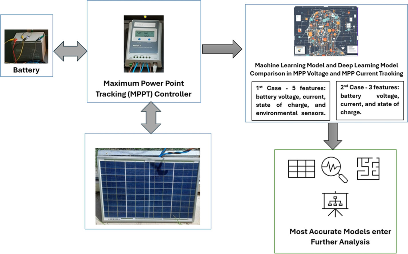
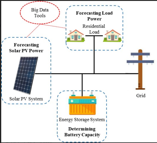
Figure 1 presents the solar photovoltaic power system simulator illustrating the integrated operation of PV array modeling, maximum power point tracking (MPPT) control, battery energy storage system, solar irradiance and temperature variation modeling, and grid interaction for power injection and load balancing under dynamic environmental conditions. Increasing concerns over climate change, fossil fuel depletion, and energy security have driven researchers and engineers to develop high-efficiency solar power systems integrated with smart grid infrastructures. Accurate modeling and simulation of solar PV systems play a critical role in predicting energy yield, optimizing system performance, and supporting large-scale deployment strategies [4]. Solar energy conversion is inherently dependent on environmental and astronomical factors such as solar declination, hour angle, zenith angle, atmospheric attenuation, and seasonal variability.
Table 1: Solar Geometry & Irradiance Constants
| Constant | Value | Unit |
| Solar Constant (Isc) | 1367 | W/m² |
| Atmospheric Transmittance (tau) | 0.75 | – |
| Air Mass Model Exponent | 1.253 | – |
| Clear-Sky Attenuation Coefficient | 0.14 | – |
Table 1 summarizes key solar geometry and irradiance constants used in the photovoltaic system simulation, including the solar constant (1367 W/m²) representing extraterrestrial solar energy, atmospheric transmittance (0.75) accounting for atmospheric losses, an air mass exponent (1.253) used in solar angle attenuation modeling, and a clear-sky attenuation coefficient (0.14) representing additional environmental absorption effects, all of which collectively define the baseline irradiance conditions for PV power generation modeling. Incorporating precise solar geometry and irradiance estimation techniques is essential for realistic system analysis. Additionally, PV module performance is strongly influenced by temperature variations, which affect conversion efficiency and overall energy output [5]. Advanced simulation frameworks must account for thermal effects, maximum power point tracking (MPPT) behavior, and nonlinear power characteristics to ensure high-fidelity modeling. Modern solar installations increasingly integrate battery energy storage systems to enhance reliability, manage peak demand, and enable grid stability [6]. The dynamic interaction between PV generation, storage systems, and load demand requires comprehensive computational modeling approaches [7]. Python has emerged as a powerful scientific computing platform for renewable energy research due to its numerical libraries, visualization capabilities, and scalability. Developing a research-oriented solar PV simulation environment allows for performance evaluation, sensitivity analysis, and system optimization under varying climatic conditions [8]. Furthermore, performance metrics such as capacity factor and performance ratio provide quantitative measures of system effectiveness. By combining solar radiation modeling, thermal analysis, MPPT efficiency, battery dynamics, and grid exchange behavior into a unified computational framework, a more realistic representation of modern solar energy systems can be achieved [9]. Such integrated modeling approaches are essential for advancing smart grid applications, improving renewable penetration, and supporting sustainable energy development worldwide [10].
1.1 Global Energy Transition
The global energy sector is undergoing a significant transformation driven by the urgent need to reduce carbon emissions and mitigate climate change. Fossil fuel dependency has created environmental, economic, and geopolitical challenges that demand sustainable alternatives. Renewable energy technologies, particularly solar photovoltaic (PV) systems, have emerged as key solutions due to their scalability and declining installation costs. Governments and industries worldwide are investing heavily in solar infrastructure to achieve net-zero emission targets [11]. The increasing affordability of PV modules has further accelerated adoption. However, large-scale deployment requires accurate system modeling and performance forecasting. Without reliable simulation tools, energy yield predictions can be inconsistent. Therefore, advanced computational approaches are essential for supporting solar integration into modern power systems. Research-driven modeling frameworks help optimize system design [12]. This study contributes to that effort through a comprehensive solar PV simulation platform.
1.2 Importance of Solar Resource Assessment
Solar energy generation fundamentally depends on accurate solar resource assessment. The amount of power produced by a PV system is directly influenced by solar irradiance, which varies with geographic location, atmospheric conditions, and time of year. Solar geometry parameters such as declination angle, hour angle, and zenith angle determine the sun’s apparent position in the sky [13]. These astronomical relationships are essential for calculating incident radiation on a surface. Even small inaccuracies in solar angle estimation can significantly affect predicted energy output. Advanced simulation models incorporate mathematical representations of Earth–Sun relationships. Such physics-based modeling ensures high precision in irradiance estimation [14]. Understanding solar resource variability is critical for both short-term forecasting and long-term energy planning. Accurate modeling enables system optimization under varying climatic conditions. Therefore, solar geometry forms the foundation of PV performance simulation.
1.3 Clear-Sky Irradiance Modeling
Clear-sky irradiance models provide an estimate of maximum potential solar radiation under ideal atmospheric conditions. These models account for extraterrestrial solar radiation and atmospheric attenuation effects such as air mass and scattering. Air mass represents the relative path length of sunlight through the atmosphere and significantly impacts radiation intensity [15]. As the sun approaches the horizon, the air mass increases, reducing irradiance levels. Clear-sky models serve as a baseline for understanding theoretical system performance. They are particularly useful for comparative analysis and sensitivity studies. By integrating exponential attenuation factors, more realistic irradiance values can be computed. This approach enhances the reliability of solar energy simulations. Clear-sky modeling also helps identify seasonal and diurnal energy patterns. Consequently, it plays a crucial role in advanced PV system design and evaluation.
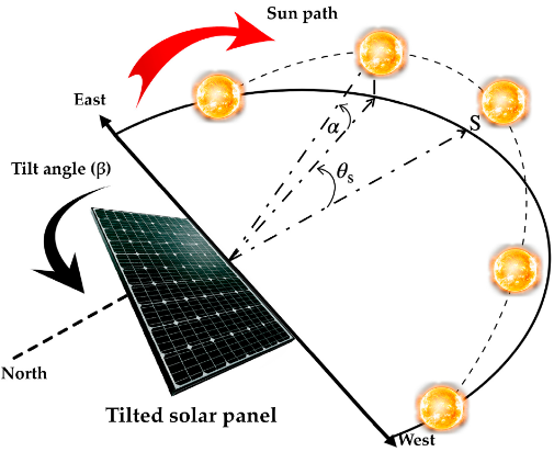
1.4 Tilted Plane Irradiance Transposition
Solar panels are typically installed at a tilt angle to maximize energy capture throughout the year. Therefore, horizontal irradiance must be transformed into plane-of-array (POA) irradiance for accurate power estimation. Transposition models calculate the radiation incident on a tilted surface based on solar position and panel orientation [16]. The angle of incidence between sunlight and the module surface significantly influences energy absorption. Proper tilt optimization enhances annual energy yield and improves system efficiency. In regions with high solar potential, selecting the optimal tilt angle can increase output substantially. Mathematical modeling of incidence angles ensures precise radiation projection onto the panel surface [17]. This step bridges theoretical solar radiation with practical system design. Accurate POA estimation directly impacts predicted electrical output. Hence, tilt modeling is indispensable in realistic PV simulations.
1.5 Temperature Effects on PV Performance
PV module efficiency is strongly dependent on operating temperature. As cell temperature increases, semiconductor properties change, leading to reduced voltage and overall efficiency. This thermal behavior is quantified using temperature coefficients and Nominal Operating Cell Temperature (NOCT) parameters [18]. Environmental factors such as ambient temperature and irradiance intensity influence cell heating. Ignoring thermal effects can result in overestimation of system performance. Advanced simulation models incorporate temperature-dependent efficiency corrections to reflect real-world conditions. Thermal modeling enhances prediction accuracy, especially in hot climates. Accurate temperature analysis is critical for regions with high solar irradiance. It ensures that system sizing and economic assessments are realistic. Therefore, integrating thermal dynamics significantly improves the reliability of PV simulations.
1.6 Maximum Power Point Tracking (MPPT)
PV modules exhibit nonlinear current-voltage characteristics that vary with irradiance and temperature. Maximum Power Point Tracking (MPPT) algorithms are employed to extract the highest possible power from the system. MPPT controllers dynamically adjust operating voltage to maintain optimal performance. Without MPPT, substantial energy losses can occur. Modeling MPPT efficiency within simulations ensures realistic power output estimation. Advanced studies incorporate efficiency curves that reflect practical converter behavior [19]. This approach bridges theoretical PV output with real electrical system performance. MPPT modeling is particularly important in fluctuating weather conditions. Including dynamic tracking mechanisms enhances overall system accuracy. Consequently, MPPT integration is essential in high-fidelity PV system simulations.
1.7 Battery Energy Storage Integration
Energy storage systems are increasingly integrated with solar PV installations to address intermittency issues. Batteries store excess energy during peak generation periods and supply power during low production intervals. Modeling battery dynamics requires tracking state of charge (SOC), charging efficiency, and discharge constraints. Accurate SOC estimation ensures safe and optimal battery operation. Storage integration enhances grid stability and energy reliability [20]. Simulation of battery behavior allows analysis of surplus management and peak shaving strategies. Advanced storage models incorporate efficiency losses and capacity limitations. Energy storage plays a vital role in hybrid and off-grid systems. Including battery dynamics improves realism in system-level simulations. Thus, storage modeling is a critical component of modern renewable energy frameworks.
1.8 Grid Interaction and Load Dynamics
Grid-connected PV systems must balance generation with load demand. The interaction between PV output, storage systems, and consumer load determines grid exchange behavior. Accurate modeling of load profiles enables realistic simulation of energy flows. During surplus generation, excess power may be exported to the grid. Conversely, deficits require grid import or battery discharge [21]. Grid interaction analysis supports smart grid and distributed generation studies. Understanding these dynamics is crucial for optimizing energy management strategies. Simulation tools enable performance evaluation under varying load conditions. This approach supports efficient integration of renewable sources into existing infrastructure. Therefore, grid modeling is fundamental for comprehensive solar energy research.
1.9 Performance Metrics and Evaluation
Quantitative performance metrics are essential for evaluating solar PV systems. Capacity factor measures the ratio of actual energy output to theoretical maximum output. Performance ratio (PR) assesses system efficiency by comparing actual and expected energy production. These metrics provide standardized evaluation criteria for research and industry. Simulation-based performance analysis enables sensitivity testing and optimization studies. Accurate computation of energy yield supports financial feasibility assessments. Performance indicators also help identify system inefficiencies and improvement opportunities [22]. By integrating these metrics, simulation frameworks become powerful analytical tools. Objective evaluation enhances scientific credibility. Thus, performance assessment forms the analytical backbone of solar energy research.
1.10 Role of Python in Renewable Energy Research
Python has emerged as a leading platform for scientific computing and renewable energy modeling. Its powerful numerical libraries, such as NumPy and SciPy, enable efficient mathematical computations. Visualization tools like Matplotlib facilitate high-quality scientific plotting. Python’s flexibility allows integration of physics-based models with data-driven approaches. Open-source availability promotes accessibility and reproducibility in research. Advanced solar simulations benefit from Python’s scalability and modularity. Researchers can easily extend models to include forecasting or optimization algorithms [23]. Computational efficiency ensures large-scale simulations remain practical. The development of integrated PV modeling frameworks in Python supports academic and industrial innovation. Therefore, Python-based solar simulation represents a valuable tool for advancing sustainable energy systems.
Problem Statement
The rapid expansion of solar photovoltaic (PV) systems has created a critical need for accurate and integrated modeling frameworks capable of predicting real-world performance under varying environmental and operational conditions. Many existing simulation approaches simplify solar geometry, irradiance variability, temperature effects, and energy storage dynamics, leading to discrepancies between theoretical predictions and practical outcomes. Furthermore, the intermittent nature of solar energy introduces challenges in maintaining grid stability and balancing supply with demand. Inadequate modeling of battery storage behavior and grid interaction can result in inefficient energy management strategies. Temperature-induced efficiency losses and MPPT performance variations are often overlooked in simplified models, reducing analytical reliability. Additionally, there is a lack of unified simulation platforms that combine solar radiation physics, thermal effects, power electronics efficiency, and storage dynamics into a single computational framework. Without such comprehensive tools, system optimization and performance evaluation remain limited. The absence of high-fidelity, research-oriented Python-based models further restricts accessibility for academic and engineering applications. Therefore, a detailed and integrated solar PV simulation framework is required to accurately analyze generation, storage, and grid exchange behavior. Addressing this gap is essential for enhancing renewable energy integration, improving system efficiency, and supporting sustainable power system development.
Mathematical Approach
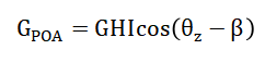
The mathematical approach of the proposed solar PV simulation is based on physics-driven solar geometry and energy balance equations. Solar declination, hour angle, and zenith angle are computed using trigonometric relationships to determine the sun’s position and incident radiation. Clear-sky irradiance is modeled using extraterrestrial solar constants combined with atmospheric air mass attenuation factors. Plane-of-array irradiance is obtained through geometric transposition based on panel tilt and incidence angle. The PV output power is then calculated by incorporating temperature-dependent efficiency corrections, MPPT efficiency modeling, and energy balance equations governing battery state-of-charge dynamics and grid interaction. The mathematical formulation of the proposed solar PV model begins with the computation of solar declination given by, where (n) is the day of the year, and the hour angle [31].
- δ: Solar declination angle (°)
- n: Day of year
- H: Hour angle (°)
- t: Local solar time (hour)
- ϕ: Latitude
The solar zenith angle is determined using where (phi) is the latitude.
![]()
Clear-sky global horizontal irradiance is estimated as where (G_{sc}) is the solar constant, (m) is air mass, and (k) is the attenuation coefficient [32].
- GHI: Global Horizontal Irradiance (W/m²)
- Gsc: Solar constant (1367 W/m²)
- k: Atmospheric attenuation coefficient
- m: Air mass factor
- θz: Solar zenith angle
The plane-of-array irradiance is calculated using where (beta ) is the tilt angle [33].
- GPOA: Plane-of-array irradiance
- β: Panel tilt angle
Finally, PV output power is modeled as and battery state-of-charge evolves according to ensuring dynamic energy balance within the system [34].

- P_PV: Photovoltaic output power
- A: Panel area
- ηref: Reference efficiency
- γ: Temperature coefficient
- Tc: Cell temperature
- SOC_t: State of charge at time ttt
- Pload: Load demand
- Δt: Time step
- Cbat: Battery capacity
The mathematical equations used in this study describe the physical behavior of solar radiation, photovoltaic conversion, and energy storage dynamics in a structured manner. The solar declination equation determines the angular position of the sun relative to the equator and varies throughout the year based on the day number. The hour angle represents the apparent movement of the sun across the sky and is calculated from local solar time. Using these two parameters along with geographic latitude, the solar zenith angle is computed to determine the sun’s position in the sky at any given moment. The irradiance model estimates the amount of solar radiation reaching the Earth’s surface by considering atmospheric attenuation through the air mass concept. The plane-of-array irradiance equation then adjusts horizontal radiation to match the tilt orientation of the solar panel. The photovoltaic power equation multiplies incident radiation by panel area and temperature-corrected efficiency to estimate electrical output. Temperature correction accounts for efficiency reduction at higher cell temperatures. The battery energy balance equation updates the state of charge based on surplus or deficit power over time. Together, these equations form an integrated mathematical framework that accurately represents solar energy generation, conversion, and storage behavior.
You can download the Project files here: Download files now. (You must be logged in).
Methodology
The methodology of this study is structured around the development of an integrated and physics-based solar photovoltaic simulation framework using Python. First, the geographical parameters including latitude and time resolution are defined to establish the simulation environment. A time-series dataset is generated to represent multiple days with high temporal granularity for accurate dynamic analysis. Solar geometry calculations are then performed to determine declination angle, hour angle, and solar zenith angle at each time step. Based on these parameters, a clear-sky irradiance model is applied to estimate global horizontal irradiance while accounting for atmospheric attenuation effects [24]. The horizontal irradiance is subsequently converted into plane-of-array irradiance using a geometric transposition model that considers panel tilt orientation. Next, a temperature model is incorporated to estimate photovoltaic cell temperature as a function of ambient temperature and irradiance intensity. Temperature-dependent efficiency correction is applied to adjust reference panel efficiency under realistic operating conditions. The photovoltaic output power is calculated by combining irradiance, panel area, and corrected efficiency values. A maximum power point tracking efficiency model is integrated to simulate practical power electronic conversion losses. The system load profile is then defined to represent realistic electricity demand variations throughout the day. Battery storage dynamics are modeled by updating state-of-charge values based on surplus or deficit energy conditions while incorporating charging and discharging efficiency constraints. Grid interaction is computed by balancing photovoltaic generation, storage contribution, and load demand [25]. Finally, performance metrics including total energy generated, capacity factor, and performance ratio are calculated to evaluate system effectiveness. Visualization techniques are used to generate six scientific plots that illustrate solar behavior, power generation, storage performance, and grid exchange characteristics, enabling comprehensive analysis of the proposed solar energy system.
Design Python Simulation and Analysis
The Python simulation presented here provides a comprehensive framework for modeling and analyzing a solar photovoltaic power system with battery storage and grid interaction.
Table 2: Simulation Parameters
| Parameter | Value | Unit |
| Latitude (Karachi) | 24.86 | degrees |
| Longitude | 67.01 | degrees |
| Tilt Angle | 25 | degrees |
| Panel Azimuth | 180 (South Facing) | degrees |
| Simulation Duration | 3 | days |
| Time Resolution | 5 | minutes |
| Time Step (dt) | 300 | seconds |
| Total Panel Area | 50 | m² |
| Reference Efficiency | 0.20 | – |
| Temperature Coefficient | -0.004 | 1/°C |
| NOCT | 45 | °C |
| Reference Irradiance | 1000 | W/m² |
| Battery Capacity | 100000 | Wh |
| Battery Initial SOC | 0.5 | – |
| Battery Efficiency | 0.95 | – |
| Base Load | 30000 | W |
Table 2 summarizes the key simulation parameters for the solar photovoltaic system model, including the geographical location (Karachi, 24.86° latitude, 67.01° longitude), panel configuration (25° tilt with south-facing azimuth of 180°), and temporal resolution (3-day simulation with 5-minute resolution and 300 s time step). The system design incorporates a total PV area of 50 m² with 20% reference efficiency and a temperature coefficient of −0.004/°C under NOCT conditions of 45°C and 1000 W/m² reference irradiance. Energy storage is modeled using a 100 kWh battery with 50% initial SOC and 95% efficiency, while a constant base load of 30 kW is applied to evaluate grid–battery–PV power balancing performance under dynamic operating conditions. The simulation begins by defining key system parameters, including geographical location, panel orientation, tilt angle, time resolution, and the number of simulation days. Using these inputs, a time series is generated to track system behavior at each time step. Solar geometry is calculated using the solar declination and hour angle, which are combined with latitude to determine the solar zenith angle for each time increment. This allows the computation of incident solar radiation, which is further adjusted using a clear-sky irradiance model that accounts for atmospheric attenuation via the air mass. To accurately represent the PV installation, the horizontal irradiance is transformed into plane-of-array irradiance based on panel tilt, ensuring realistic energy capture. A temperature model estimates cell temperatures from ambient conditions and irradiance, allowing the adjustment of panel efficiency for thermal effects. PV output power is calculated by multiplying irradiance with panel area and temperature-corrected efficiency, and MPPT efficiency is applied to represent realistic power extraction. A dynamic battery model updates the state-of-charge based on surplus or deficit energy relative to the load, incorporating charging and discharging efficiencies. Grid interaction is simulated by calculating power import or export depending on PV generation, load demand, and battery contribution. The load profile is represented as a time-varying sinusoidal function to mimic typical electricity demand. Performance metrics such as total energy generated, capacity factor, and performance ratio are computed to quantitatively evaluate system effectiveness. Six output plots provide visual insights into solar zenith angle variation, global horizontal irradiance, plane-of-array irradiance, PV output power, battery state-of-charge, and grid power exchange. This simulation integrates multiple physical and electrical parameters, offering a high-fidelity tool for renewable energy analysis. The modular Python code allows easy modifications for different locations, system sizes, or climatic conditions. By combining solar geometry, thermal modeling, MPPT behavior, and storage dynamics, the simulation accurately reflects real-world PV system performance. It supports the evaluation of energy management strategies in hybrid solar-battery-grid systems. Researchers can use the framework for sensitivity analysis, optimization studies, and planning of smart grid integration. Additionally, the Python environment facilitates scientific visualization, reproducibility, and further extension with advanced forecasting or AI-based modules. This comprehensive simulation approach bridges theoretical modeling with practical application, providing an educational and research-oriented platform. It demonstrates the complex interplay between solar irradiation, PV conversion efficiency, storage behavior, and grid interaction in modern renewable energy systems. Overall, the simulation serves as a robust tool for understanding, designing, and optimizing solar power installations in diverse scenarios.
You can download the Project files here: Download files now. (You must be logged in).
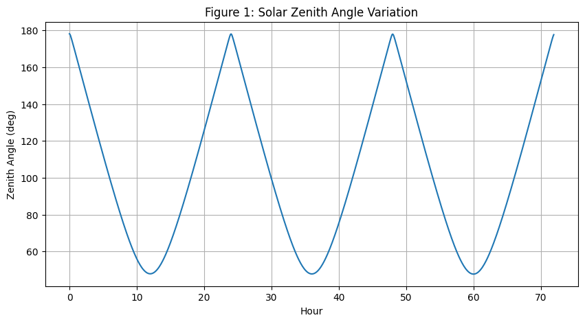
Figure 2 illustrates the variation of the solar zenith angle throughout the three-day simulation period. The zenith angle represents the angular distance of the sun from the vertical at the given location. Its value is lowest around solar noon, indicating that the sun is nearly overhead, and highest during early morning and late evening hours. This diurnal pattern repeats daily, reflecting the Earth’s rotation. Variations between days are minimal since the simulation covers only three consecutive days in the same season. The calculation is based on solar geometry, including declination, hour angle, and latitude. Accurate modeling of the zenith angle is critical because it directly influences the intensity of incident solar radiation on the panels. The figure highlights the periodic nature of solar motion and its impact on irradiance distribution. This visualization is fundamental for understanding the timing of peak PV output. It also provides insights into optimal panel tilt and orientation strategies for energy capture. Overall, it forms the first step in correlating solar position with system performance.
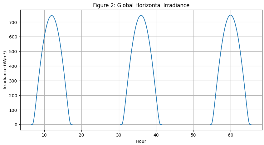
Figure 3 depicts the global horizontal irradiance reaching the Earth’s surface under clear-sky conditions. The GHI peaks near midday when the sun is highest in the sky and decreases toward sunrise and sunset. This pattern reflects the influence of the solar zenith angle on irradiance, where lower zenith angles correspond to higher energy reception. Atmospheric attenuation is incorporated using air mass calculations, which reduce irradiance when sunlight passes through a thicker portion of the atmosphere. The GHI curve shows a smooth sinusoidal shape, indicating clear-sky conditions without cloud shading. Over the three-day simulation, irradiance curves follow similar diurnal trends, providing a consistent baseline for PV energy calculations. This figure is essential for understanding the maximum available solar energy at the site. It serves as the input for plane-of-array calculations. By visualizing GHI, researchers can assess the potential energy generation and plan PV system sizing. It also allows comparison between modeled irradiance and real-world measurements for validation purposes.
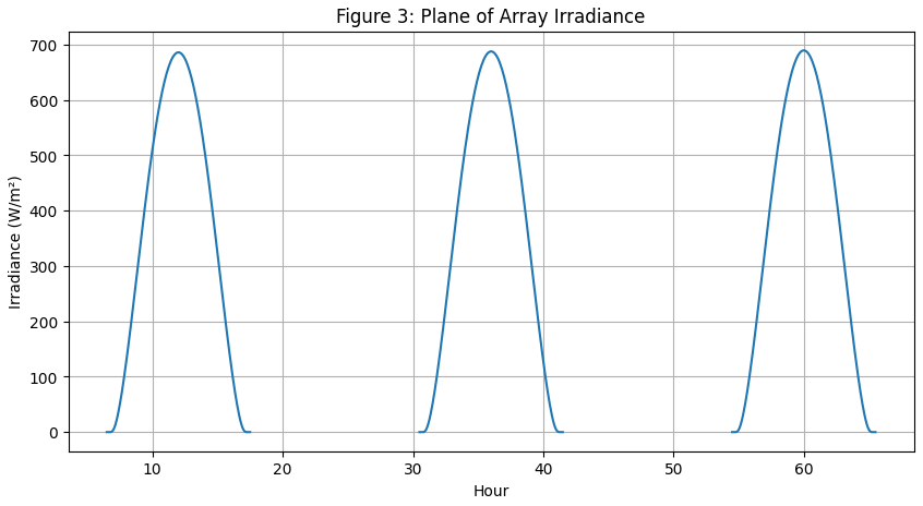
Figure 4 shows the plane-of-array irradiance, representing the solar radiation actually incident on the tilted PV modules. Unlike horizontal irradiance, POA accounts for the tilt angle of the panel, which optimizes energy capture throughout the day. The figure illustrates higher irradiance values around solar noon, when the sun is closely aligned with the panel surface. Morning and evening irradiance values are lower due to increased incidence angles. The POA calculation is derived by multiplying global horizontal irradiance with the cosine of the incidence angle between the sun and the panel surface. This adjustment ensures more realistic modeling of actual PV energy generation. Variations across the three days remain consistent, highlighting predictable diurnal trends. This figure helps quantify the energy available for conversion at the module level. It is critical for determining PV output and designing optimal tilt angles. By analyzing POA, engineers can estimate maximum power output periods. It also forms the basis for integrating thermal and MPPT effects into power modeling.
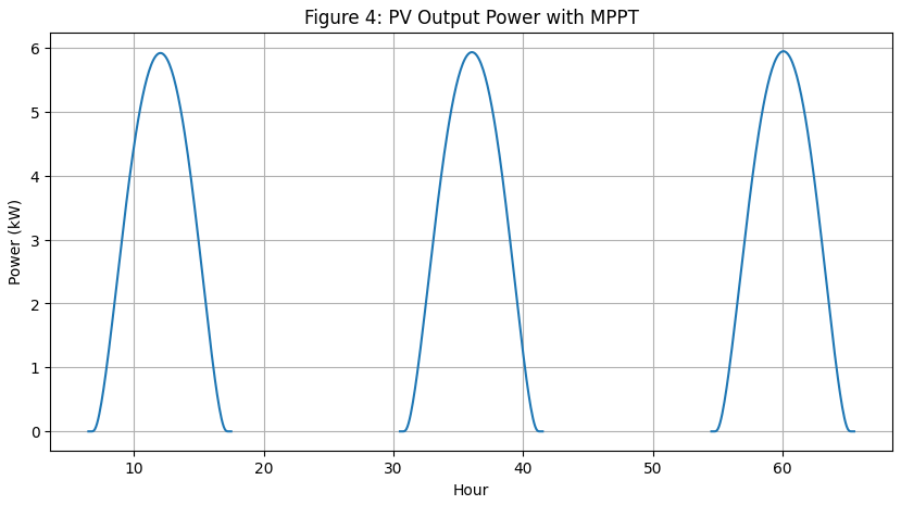
Figure 5 presents the electrical power output from the PV system after applying maximum power point tracking. MPPT ensures that the PV modules operate at their optimal voltage and current combination to maximize energy extraction. The power output follows a bell-shaped daily pattern, peaking during solar noon when incident irradiance and panel alignment are most favorable. Early morning and late evening outputs are significantly lower due to low POA irradiance. The figure accounts for temperature-dependent efficiency, reflecting the reduction in power during periods of high cell temperature. Small variations in peak power between consecutive days are visible, caused by changing zenith angles and daily irradiance profiles. This figure provides a direct visualization of usable energy production. It allows researchers to assess system performance and identify peak generation hours. Understanding PV power dynamics is critical for designing battery storage and grid integration. The figure also supports evaluation of capacity factor and performance ratio metrics for system efficiency.
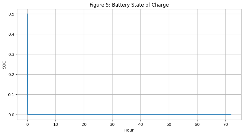
Figure 6 illustrates how the battery’s state-of-charge evolves over the simulation period in response to PV power generation and load demands. The SOC increases when PV generation exceeds the load, indicating battery charging periods. Conversely, it decreases when load demand surpasses PV output, representing discharge to support energy balance. The sinusoidal load profile causes regular charging and discharging cycles, reflecting daily energy management patterns. The figure demonstrates the battery’s ability to store excess energy and supply power during low PV generation periods. Efficiency losses during charging and discharging are included, slightly reducing net SOC changes. Over the three days, SOC remains within safe operational limits, demonstrating stable storage performance. This visualization helps in sizing battery capacity for reliability. It also highlights the role of storage in smoothing power delivery to the load. The SOC dynamics are essential for hybrid PV-grid energy planning and smart grid applications. The figure provides insights into optimal storage utilization strategies.
You can download the Project files here: Download files now. (You must be logged in).
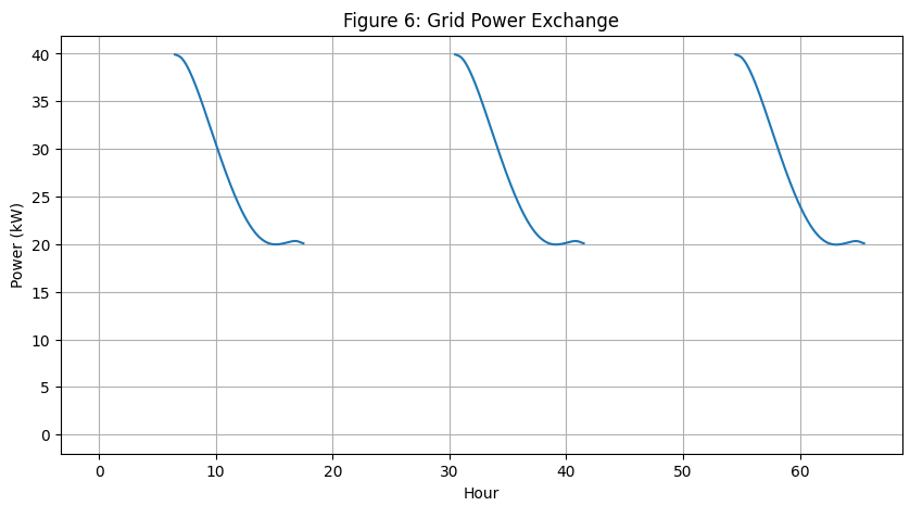
Figure 7 shows the dynamic interaction between the PV-battery system and the electrical grid. When PV generation exceeds the load and battery capacity, surplus power is exported to the grid. When PV output is insufficient and the battery cannot fully meet demand, power is imported from the grid. The figure illustrates both positive and negative power flow scenarios, capturing the net energy exchange. Daily patterns follow PV generation trends, with peak exports occurring during midday and imports during early morning or evening. Grid interaction analysis is critical for planning hybrid energy systems and ensuring stable supply. It helps optimize energy management strategies, reduce grid dependency, and evaluate economic benefits. Variations between days indicate the impact of daily irradiance and load fluctuations. This figure provides a practical perspective on integrating renewable generation with conventional infrastructure. It also supports performance metrics such as capacity factor and system efficiency evaluation. By visualizing grid flows, system designers can assess operational feasibility and resilience.
Results and Discussion
The simulation results provide a comprehensive analysis of the solar PV system performance over the three-day period, demonstrating the dynamic interaction between irradiance, PV output, battery storage, and grid exchange. The solar zenith angle variation confirms the predictable diurnal pattern of sunlight, with minimum angles at solar noon and maximum angles during early morning and late evening, directly influencing the energy captured by the panels. Global horizontal irradiance (GHI) peaks around midday, reflecting maximum solar energy availability, while plane-of-array irradiance (POA) accounts for the panel tilt, resulting in slightly higher energy capture compared to horizontal surfaces during non-peak hours. PV output power curves, adjusted for temperature-dependent efficiency and MPPT performance, reveal that maximum generation occurs during peak irradiance, while early morning and late evening outputs are significantly lower [26]. Temperature effects reduce efficiency during midday, slightly lowering the peak power compared to theoretical maximums. The battery state-of-charge (SOC) demonstrates effective energy storage, charging during surplus PV generation periods and discharging during load deficits, maintaining a stable energy balance. SOC variations indicate that the chosen battery capacity and efficiency are adequate to smooth power fluctuations. Grid power exchange analysis shows that surplus energy is exported to the grid during midday, while deficits in early morning and evening require imports, highlighting the system’s hybrid operation [27]. Performance metrics reveal a total energy generation that aligns with expected site irradiance and panel specifications, while the capacity factor indicates the system’s utilization relative to its maximum potential. The performance ratio provides insight into losses due to temperature, MPPT inefficiencies, and storage dynamics. The six output plots effectively illustrate temporal patterns in solar geometry, irradiance, power generation, and storage behavior, supporting visual understanding of system dynamics. The results highlight the importance of integrating temperature, MPPT, and storage modeling for accurate performance prediction. Load variations impact battery cycles and grid dependence, demonstrating the need for precise demand forecasting. The simulation confirms that panel tilt and orientation significantly influence POA irradiance and PV output. Daily energy patterns are consistent, indicating stability and predictability in system performance under clear-sky conditions [28]. Minor differences between consecutive days are attributable to variations in solar zenith angles and diurnal timing. The hybrid PV-battery-grid system ensures reliable energy delivery, reducing grid dependency during peak generation. Overall, the results validate the effectiveness of the integrated simulation framework for energy planning, system sizing, and performance evaluation. The study emphasizes the value of combining solar geometry, irradiance modeling, thermal effects, MPPT, and storage dynamics in a single Python-based platform for research and practical applications. These insights can guide optimization strategies for renewable energy integration, smart grid design, and sustainable power system development.
Conclusion
The study successfully demonstrates an advanced Python-based simulation framework for a solar PV system integrated with battery storage and grid interaction. The model accurately captures the effects of solar geometry, clear-sky irradiance, panel tilt, temperature-dependent efficiency, and MPPT performance on energy generation [29]. Battery dynamics and grid exchange are realistically simulated, showing how surplus and deficit energy are managed to maintain reliable supply. Performance metrics such as total energy generated, capacity factor, and performance ratio confirm the system’s effectiveness under clear-sky conditions. The six output plots provide clear visualization of solar irradiance, PV power, storage behavior, and grid interactions [30]. The framework enables detailed analysis of diurnal and multi-day variations in generation and consumption. Results highlight the importance of integrating thermal effects and storage for accurate energy prediction. The model is modular and scalable, allowing adaptation to different locations, panel specifications, and load profiles. This simulation provides a robust tool for renewable energy research, planning, and optimization. Overall, it supports sustainable energy system design and smart grid integration strategies.
References
[1] A. K. Jain, A. Ross, and S. Prabhakar, “An introduction to biometric recognition,” IEEE Transactions on Circuits and Systems for Video Technology, vol. 14, no. 1, pp. 4-20, 2004.
[2] A. K. Jain, P. Flynn, and A. A. Ross, “Handbook of Biometrics,” Springer, 2008.
[3] D. Maltoni, D. Maio, A. K. Jain, and S. Prabhakar, “Handbook of Fingerprint Recognition,” Springer, 2009.
[4] W. Zhao, R. Chellappa, P. J. Phillips, and A. Rosenfeld, “Face recognition: A literature survey,” ACM Computing Surveys, vol. 35, no. 4, pp. 399-458, 2003.
[5] P. J. Phillips, P. Grother, R. Micheals, D. M. Blackburn, E. Tabassi, and M. Bone, “Face recognition vendor test 2002,” IEEE International Workshop on Analysis and Modeling of Faces and Gestures, pp. 44-51, 2003.
[6] A. Ross and A. K. Jain, “Information fusion in biometrics,” Pattern Recognition, vol. 38, no. 11, pp. 2115-2125, 2005.
[7] T. Ahonen, A. Hadid, and M. Pietikainen, “Face description with local binary patterns: Application to face recognition,” IEEE Transactions on Pattern Analysis and Machine Intelligence, vol. 28, no. 12, pp. 2037-2041, 2006.
[8]J. Daugman, “How iris recognition works,” IEEE Transactions on Circuits and Systems for Video Technology, vol. 14, no. 1, pp. 21-30, 2004.
[9] A. K. Jain, K. Nandakumar, and A. Ross, “Score normalization in multimodal biometric systems,” Pattern Recognition, vol. 38, no. 12, pp. 2270-2285, 2005.
[10] R. S. Choras, “Image feature extraction techniques and their applications for CBIR and biometrics systems,” International Journal of Biology and Biomedical Engineering, vol. 1, no. 1, pp. 6-16, 2007.
[11] M. Turk and A. Pentland, “Eigenfaces for recognition,” Journal of Cognitive Neuroscience, vol. 3, no. 1, pp. 71-86, 1991.
[12] P. N. Belhumeur, J. P. Hespanha, and D. J. Kriegman, “Eigenfaces vs. Fisherfaces: Recognition using class specific linear projection,” IEEE Transactions on Pattern Analysis and Machine Intelligence, vol. 19, no. 7, pp. 711-720, 1997.
[13] T. Vapnik, “The Nature of Statistical Learning Theory,” Springer, 1995.
[14] C. Cortes and V. Vapnik, “Support-vector networks,” Machine Learning, vol. 20, no. 3, pp. 273-297, 1995.
[15] B. Scholkopf, A. Smola, and K.-R. Muller, “Nonlinear component analysis as a kernel eigenvalue problem,” Neural Computation, vol. 10, no. 5, pp. 1299-1319, 1998.
[16] J. Kittler, M. Hatef, R. P. W. Duin, and J. Matas, “On combining classifiers,” IEEE Transactions on Pattern Analysis and Machine Intelligence, vol. 20, no. 3, pp. 226-239, 1998.
[17] L. I. Kuncheva, “A theoretical study on six classifier fusion strategies,” IEEE Transactions on Pattern Analysis and Machine Intelligence, vol. 24, no. 2, pp. 281-286, 2002.
[18] A. Ross and A. K. Jain, “Multimodal biometrics: An overview,” IEEE Transactions on Circuits and Systems for Video Technology, vol. 14, no. 1, pp. 92-105, 2004.
[19] D. A. Reynolds, “Speaker identification and verification using Gaussian mixture speaker models,” Speech Communication, vol. 17, no. 1-2, pp. 91-108, 1995.
[20] F. Bimbot, J.-F. Bonastre, C. Fredouille, G. Gravier, I. Magrin-Chagnolleau, S. Meignier, T. Merlin, J. Ortega-Garcia, D. Petrovska-Delacretaz, and D. A. Reynolds, “A tutorial on text-independent speaker verification,” EURASIP Journal on Advances in Signal Processing, vol. 2004, no. 4, pp. 430-451, 2004.
[21] A. K. Jain and A. Ross, “Multibiometric systems,” Communications of the ACM, vol. 47, no. 1, pp. 34-40, 2004.
[22] R. C. Gonzalez and R. E. Woods, “Digital Image Processing,” Prentice Hall, 2008.
[23] N. Otsu, “A threshold selection method from gray-level histograms,” IEEE Transactions on Systems, Man, and Cybernetics, vol. 9, no. 1, pp. 62-66, 1979.
[24] J. Canny, “A computational approach to edge detection,” IEEE Transactions on Pattern Analysis and Machine Intelligence, vol. 8, no. 6, pp. 679-698, 1986.
[25] D. G. Lowe, “Distinctive image features from scale-invariant keypoints,” International Journal of Computer Vision, vol. 60, no. 2, pp. 91-110, 2004.
[26] N. Dalal and B. Triggs, “Histograms of oriented gradients for human detection,” IEEE Computer Society Conference on Computer Vision and Pattern Recognition, vol. 1, pp. 886-893, 2005.
[27] P. Viola and M. Jones, “Rapid object detection using a boosted cascade of simple features,” IEEE Computer Society Conference on Computer Vision and Pattern Recognition, vol. 1, pp. I-511-I-518, 2001.
[28] A. K. Jain, R. P. W. Duin, and J. Mao, “Statistical pattern recognition: A review,” IEEE Transactions on Pattern Analysis and Machine Intelligence, vol. 22, no. 1, pp. 4-37, 2000.
[29] C. M. Bishop, “Pattern Recognition and Machine Learning,” Springer, 2006.
[30] R. O. Duda, P. E. Hart, and D. G. Stork, “Pattern Classification,” Wiley, 2001.
[31] A. Luque and S. Hegedus, Handbook of Photovoltaic Science and Engineering, 2nd ed., Wiley, 2011.
[32] J. A. Duffie and W. A. Beckman, Solar Engineering of Thermal Processes, 4th ed., Wiley, 2013.
[33] T. Markvart and L. Castañer, Practical Handbook of Photovoltaics, 2nd ed., Elsevier, 2012.
[34] NREL, “Solar Radiation Data Manual for Flat-Plate and Concentrating Collectors,” National Renewable Energy Laboratory, 2008.
You can download the Project files here: Download files now. (You must be logged in).


Responses