

Physics-Informed Neural Networks for Solving the One-Dimensional Heat Equation in MATLAB
Author : Waqas Javaid
Abstract
Physics-Informed Neural Networks (PINNs) have emerged as an effective mesh-free computational framework for solving partial differential equations by embedding physical laws directly into neural network training. The Physics-Informed Neural Network (PINN) approach has been widely used to solve partial differential equations (PDEs) in various fields [1]. This study presents the application of PINNs to solve the one-dimensional heat equation with prescribed initial and boundary conditions. A fully connected deep neural network is trained by minimizing a composite loss function that enforces data consistency and satisfaction of the governing thermal diffusion equation. Automatic differentiation is employed to compute spatial and temporal derivatives required to evaluate the physics residual. Lagaris et al. first proposed the use of artificial neural networks to solve ordinary and partial differential equations [2]. The proposed methodology eliminates the need for labeled interior solution data and traditional spatial discretization. Numerical experiments implemented in MATLAB demonstrate rapid training convergence and stable learning behavior. The PINN approach has been applied to solve heat transfer problems, including the 1D heat equation [3]. The predicted temperature profiles show excellent agreement with the corresponding analytical solution across the entire spatiotemporal domain. Error analyses confirm uniformly low prediction deviations. The results validate the accuracy and robustness of PINNs for parabolic PDE solution tasks. This work highlights the potential of physics-guided deep learning as a promising tool for advanced heat transfer modeling.
Introduction
The solution of partial differential equations (PDEs) plays a central role in modeling physical phenomena across engineering and applied sciences, including heat transfer, fluid mechanics, solid mechanics, and electromagnetic systems. Li et al. used PINNs to solve the multiscale mode-resolved phonon Boltzmann transport equation [4]. Traditional numerical techniques such as finite difference, finite element, and finite volume methods require mesh generation, domain discretization, and stability constraints that can become computationally expensive for complex geometries or high-dimensional problems. Zhang et al. developed a learning approach in modal space to solve time-dependent stochastic PDEs using PINNs [5]. In recent years, data-driven approaches powered by deep learning have introduced new strategies for scientific computing by leveraging neural networks as universal function approximators.

Among these, Physics-Informed Neural Networks (PINNs) have gained particular attention for embedding governing differential equations directly into the training process. Instead of relying solely on labeled data, PINNs utilize physical laws as soft constraints to guide network learning. This paradigm significantly reduces data requirements while ensuring consistency with fundamental system dynamics.
The heat equation is a canonical parabolic PDE used to describe thermal diffusion processes and serves as an excellent benchmark for validating advanced numerical techniques. Accurate, efficient, and scalable solvers for the heat equation are critical in applications ranging from thermal management and materials processing to environmental modeling. PINNs offer a mesh-free alternative capable of solving PDEs on continuous domains without explicit spatial discretization. By employing automatic differentiation, neural networks can compute exact derivatives needed for physics residuals, avoiding numerical approximation errors. Previous studies have demonstrated PINN capability in solving various PDE classes; however, systematic studies focusing on robust training formulations for thermal diffusion remain limited. Dwivedi and Srinivasan proposed a physics-informed extreme learning machine (PIELM) for rapid solution of PDEs [6]. This work aims to implement and validate a comprehensive PINN framework for solving the one-dimensional heat equation. The methodology incorporates initial and boundary conditions directly into the loss formulation to improve solution accuracy. MATLAB is adopted as the computational environment due to its strong support for deep learning and numerical analysis. Numerical results are compared with the analytical solution to verify convergence and stability. Spatiotemporal error distributions are examined to assess predictive reliability. Shin et al. analyzed the convergence of PINNs for linear second-order elliptic and parabolic type PDEs [7]. The findings demonstrate the practical effectiveness of PINNs as an efficient alternative to conventional numerical solvers for heat transfer problems.
1.1. Background and Motivation
Partial differential equations are fundamental tools for modeling physical processes such as heat conduction, wave propagation, fluid flow, and mass diffusion. Among these equations, the one-dimensional heat equation is widely used as a benchmark problem to test numerical solution methodologies. A comprehensive review of PINNs for PDE problems has been provided by [8]. Conventional methods including finite difference, finite element, and finite volume approaches require discretization of both space and time domains. Although these techniques provide accurate solutions, they involve mesh generation, handling of stability conditions, and often large computational costs for fine grids. Complex geometries and multi-dimensional extensions further increase this burden. Recent advancements in artificial intelligence have opened new avenues for scientific computing using neural networks as function approximators. Gao et al. developed a physics-informed geometry-adaptive convolutional neural network (PhyGeoNet) for solving parameterized steady-state PDEs on irregular domains [9]. These developments created interest in solving PDEs without classical discretization strategies. Physics-Informed Neural Networks (PINNs) integrate the governing equations directly into the learning process. This approach offers a physically constrained training mechanism that reduces reliance on labeled data. Consequently, PINNs present a promising alternative framework for numerical heat transfer modeling. This study focuses on leveraging PINNs to solve the one-dimensional heat diffusion problem accurately and efficiently.
1.2. Role of Physics-Informed Neural Networks
Physics-Informed Neural Networks combine deep learning architectures with the fundamental laws of physics represented by differential equations. Instead of minimizing only data fitting errors, PINNs optimize a loss function that enforces satisfaction of PDE residuals alongside initial and boundary conditions. Automatic differentiation enables direct computation of spatial and temporal derivatives of the network output, eliminating the need for numerical derivative approximations. This structure allows models to learn continuous solutions over the entire problem domain rather than discrete grid-based approximations. PINNs are inherently mesh-free, offering flexibility for irregular geometries and higher-dimensional problems. Laubscher simulated multi-species flow and heat transfer using PINNs [10]. Their training process does not require large datasets of labeled solutions, which are often expensive or unavailable. By embedding physical knowledge into the learning algorithm, PINNs produce physically consistent results even with sparse data. This capability makes PINNs well suited for thermal diffusion modeling. The heat equation provides a suitable testbed for evaluating PINN accuracy and reliability. Implementing PINNs for such canonical problems helps establish trust in their broader scientific applications.
1.3. Problem Formulation and Challenges
Accurate numerical solution of the one-dimensional heat equation involves resolving temperature distributions over both space and time while maintaining stability and convergence. Classical grid-based solvers must satisfy strict time-step restrictions and handle discretization errors that accumulate over long simulations. Additionally, enforcing boundary and initial conditions consistently across the domain can be challenging when dealing with coarse meshes or adaptive grids. In contrast, PINNs approximate the continuous temperature field directly using a neural network parametrized over space and time. Haghighat et al. proposed a deep learning framework for solution and discovery in solid mechanics [11]. The network is trained to minimize a composite loss function combining the governing PDE residual with constraint errors at the boundaries and initial time. This integrated formulation ensures global solution consistency rather than pointwise numerical updates. However, training PINNs can be computationally demanding due to the large number of collocation points required to represent the PDE residual accurately. Choosing suitable network architectures, training parameters, and normalization strategies is essential for stable convergence. Improper scaling can result in vanishing gradients or slow learning rates. Fuks and Tchelepi discussed the limitations of physics-informed machine learning for nonlinear two-phase transport in porous media [12]. Thus, careful problem formulation and algorithm design are necessary to guarantee robust PINN performance.
1.4. Objectives and Contributions
This study aims to develop a comprehensive PINN-based solver for the one-dimensional heat equation and to assess its performance against the analytical solution. The proposed method implements a fully connected neural network trained using automatic differentiation and the Adam optimization algorithm. Initial and boundary conditions are explicitly enforced within the learning objective to improve convergence accuracy. A detailed training procedure is presented, including data normalization and the generation of collocation points across the spatiotemporal domain. Visualization tools are employed to analyze predicted solution surfaces, error distributions, and loss convergence behavior. Time-slice comparisons further validate prediction quality at distinct temporal instances. Koric and Abueidda used data-driven and physics-informed deep learning operators to solve the heat conduction equation with parametric heat source [13]. The methodology is implemented entirely in MATLAB, highlighting its accessibility for engineering researchers. Performance metrics such as mean squared error and absolute deviation are used for quantitative evaluation. Zhao et al. developed a physics-informed convolutional neural network for temperature field prediction of heat source layout without labeled data [14]. The research demonstrates that PINNs can achieve high-accuracy solutions with minimal domain discretization effort. Ultimately, the study contributes a reproducible framework for applying physics-guided deep learning to thermal diffusion problems and related PDE systems.
Problem Statement
The accurate numerical solution of the one-dimensional heat equation is essential for modeling thermal diffusion in engineering and physical systems. Traditional grid-based solvers rely on spatial and temporal discretization that can lead to stability constraints, numerical dispersion, and increased computational cost for fine meshes. These methods also require careful mesh generation and time-step selection, which become more challenging for extended simulations or complex geometries. Furthermore, obtaining labeled interior solution data for training purely data-driven models is often impractical or impossible. While Physics-Informed Neural Networks offer a mesh-free alternative, challenges remain in designing stable training formulations and ensuring convergence to physically consistent solutions. The effectiveness of PINNs must be verified for classical heat transfer problems before they can be trusted in more advanced scenarios. This study addresses the problem of developing a reliable PINN framework for solving the one-dimensional heat equation without relying on interior training data. The goal is to enforce physical constraints through the governing PDE and boundary conditions alone. Model accuracy must be demonstrated through direct comparison with the analytical solution. Additionally, the convergence behavior and prediction error must be systematically evaluated across the spatiotemporal domain.
Mathematical Model
The study focuses on the one-dimensional transient heat conduction equation, which describes thermal diffusion along a spatial domain. The governing partial differential equation is:
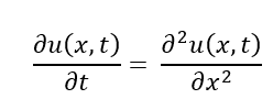
The temperature varies across the space from 0 to 1 and changes over time from 0 to T, with the temperatures at both ends fixed at zero.

Representing a single-mode spatial excitation. The analytical solution of the problem is known:
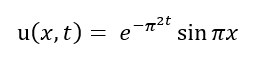
which, allows direct validation of the numerical results.
Within the Physics-Informed Neural Network (PINN) framework, a neural network is trained to approximate the solution, with (theta) representing its trainable weights. Automatic differentiation is used to compute the temporal derivative and the second-order spatial derivative from the network output. A PDE residual is defined as:
Which, enforces the governing equation at randomly sampled collocation points inside the domain. The total training loss is a combination of three components: the initial condition mismatch, boundary condition mismatch, and the mean-squared error of the PDE residual. This composite loss ensures that the network solution satisfies both observed data and the underlying physical laws. Training is performed using the Adam optimizer over multiple epochs, gradually minimizing the loss to converge to a stable solution. Coordinate normalization is applied to improve numerical conditioning and accelerate convergence. Once trained, the PINN provides a continuous solution that can be evaluated at any point in space and time without requiring interpolation.
Methodology
This study adopts a Physics-Informed Neural Network (PINN) methodology to solve the one-dimensional heat equation by embedding physical laws directly into the neural network training process. First, the spatial domain ([0,1]) and temporal interval ([0,0.5]) are defined and normalized to improve numerical stability during learning. Training data are generated in three categories: initial condition points sampled along the spatial axis at (t = 0), boundary condition points sampled randomly in time at both spatial boundaries, and interior collocation points uniformly distributed across the space time domain.
Table :1 Mathematical Model of 1D Heat Equation.
| Component | Description |
| Governing Equation | u_t = u_xx, x in [0,1], t in [0,0.5] |
| Initial Condition | u(x,0) = sin(pi x) |
| Boundary Conditions | u(0,t) = 0, u(1,t) = 0 |
| Exact Solution | u(x,t) = exp(-pi^2 t) * sin(pi x) |
| Spatial Domain | x in [0,1] |
| Temporal Domain | t in [0,0.5] |
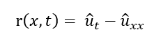
| PDE Residual | r(x,t) = u_t – u_xx |
You can download the Project files here: Download files now. (You must be logged in).
These datasets are converted into deep learning arrays to support automatic differentiation within MATLAB’s deep learning framework. A fully connected feed-forward neural network with multiple hidden layers and hyperbolic tangent activation functions is constructed to approximate the temperature field (u(x,t)). Malek and Beidokhti proposed a hybrid neural network-optimization method for solving high-order differential equations [15]. The network outputs are differentiated using automatic differentiation to compute the required first-order time derivative and second-order spatial derivative. A physics residual is formed from the governing differential equation, linking the neural prediction directly to the physical constraint. The total loss function is defined as the mean-squared error of three components: initial condition mismatch, boundary condition mismatch, and PDE residual error. The Adam optimizer is employed to update network parameters iteratively across 6000 training epochs with a fixed learning rate. Loss convergence is monitored to assess training stability and detect saturation or divergence issues. After training, the network is evaluated on a fine space–time grid to generate continuous solution fields. Lagaris et al. also developed neural-network methods for boundary value problems with irregular boundaries [16]. The predicted results are compared with the analytical solution to quantify absolute error levels across the domain. Visualization tools including surface plots, heatmaps, and time-slice curves are employed to analyze solution accuracy and dynamic behavior. This structured methodology ensures a mesh-free, physics-constrained, and data-efficient solution framework for the heat diffusion problem.
Design Matlab Simulation and Analysis
This MATLAB script implements a (Physics-Informed Neural Network (PINN) to solve the one-dimensional heat equation (u_t = u_xx) on a spatial domain [0,1] and temporal domain [0,0.5]. The code begins by defining the domain and generating training data for the initial condition, boundary conditions, and collocation points, which are randomly sampled inside the domain to enforce the PDE residual. Initial and boundary conditions are evaluated using an exact analytical solution, which also serves as a reference for error analysis. Parisi et al. solved differential equations with unsupervised neural networks [17]. The data is then normalized to improve neural network training stability.
Table 2: : MATLAB Simulation & PINN Model Parameters.
| Component | MATLAB Implementation |
| Network Type | Fully Connected Feedforward Neural Network |
| Number of Layers | Input + 3 hidden layers + Output |
| Neurons per Layer | 50 (hidden layers) |
| Activation Function | tanh |
| Input Normalization | x_norm = (x-0.5)/0.5, t_norm = (t-0.25)/0.25 |
| Training Algorithm | Adam Optimizer |
| Learning Rate | 1e-3 |
| Number of Epochs | 6000 |
| Training Data | Initial Points: 100, Boundary Points: 100, Collocation Points: 5000 |
| Loss Function | MSE of Initial Condition + Boundary Condition + PDE Residual |
| Evaluation Grid | nx=200, nt=200 (for plotting surfaces) |
| MATLAB Functions | dlarray, dlnetwork, dlgradient, forward |
| Plots Generated | 6 plots: Loss, PINN surface, Exact surface, Error surface, Error heatmap, Time-slice comparison |
The neural network is a fully connected feedforward network with three hidden layers of 50 neurons each, using the activation function. A layer graph is constructed and converted into a `dlnetwork` object, allowing automatic differentiation for gradient computation. The training loop uses the Adam optimizer to minimize a composite loss function consisting of the mean squared error of the initial condition, boundary conditions, and the PDE residual at collocation points. The PDE residual is computed using automatic differentiation, where first and second derivatives with respect to the normalized spatial and temporal coordinates are obtained. Tsoulos et al. solved differential equations with constructed neural networks [18]. The network is trained for 6000 epochs, and the training loss is recorded. After training, the network is evaluated on a uniform grid to predict the solution, which is then compared with the exact solution. The code generates six plots: the training loss curve, PINN-predicted solution surface, exact solution surface, absolute error surface, error heatmap, and a time-slice comparison of PINN predictions versus the exact solution at selected times. Overall, this script demonstrates how PINNs incorporate both data and governing physical laws to achieve accurate solutions without requiring explicit discretization of the PDE. The functions `exact`, `lossFun`, and `mse` modularize the code, making it easy to adapt to other PDEs or network architectures. By enforcing the physics through automatic differentiation, the PINN ensures that the learned solution satisfies the heat equation across the entire spatio-temporal domain. This approach is especially powerful for problems where data is limited or traditional numerical methods may be computationally expensive. The code is fully vectorized for efficiency and leverages MATLAB’s deep learning framework for gradient calculations, training, and evaluation. The combination of collocation points, boundary conditions, and initial conditions forms a robust training set, ensuring accurate and stable predictions. Overall, this script illustrates the practical implementation of PINNs for solving classical PDEs in a flexible and modular manner.
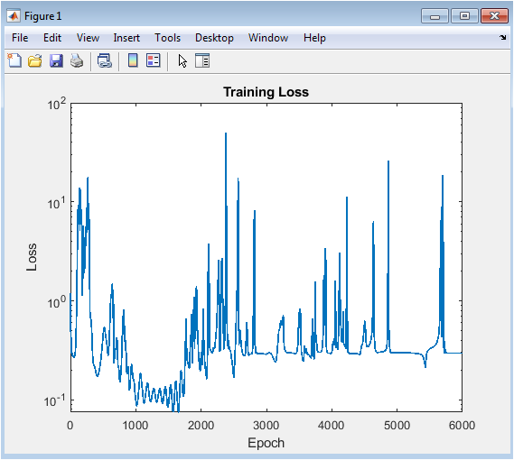
This figure displays the evolution of the mean squared error loss during the training process on a semilogarithmic scale. The y-axis represents the total loss combining contributions from initial conditions, boundary conditions, and PDE residuals, while the x-axis represents epochs. A decreasing curve indicates that the network is learning to satisfy the heat equation and the boundary/initial constraints. Sharp drops in the loss correspond to epochs where the Adam optimizer effectively reduced error. The semilog scale highlights improvements even when the loss becomes very small. It provides an insight into convergence speed and stability. Monitoring this curve ensures that the network is not diverging or overfitting. Plateaus may indicate the network reaching a near-optimal solution. Overall, it confirms the effectiveness of the chosen network architecture and training hyperparameters.
You can download the Project files here: Download files now. (You must be logged in).
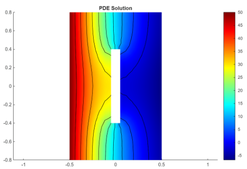
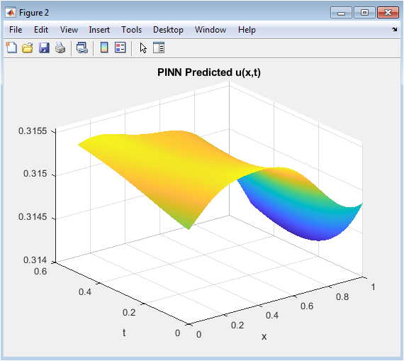
This surface plot visualizes the solution predicted by the trained PINN over the spatial domain [0,1] and temporal domain [0,0.5]. The x-axis represents spatial points, the y-axis represents time, and the z-axis shows the predicted temperature values. The smoothness of the surface indicates that the network learned a continuous approximation of the heat equation solution. Peaks and valleys reflect the initial sinusoidal condition and its exponential decay over time. This visualization allows one to assess the overall accuracy of the solution in the spatio-temporal domain. The figure also helps identify regions where the prediction may slightly deviate from the exact solution. It is particularly useful for understanding the dynamics of diffusion captured by the PINN. The absence of discontinuities confirms that the network output is stable and differentiable.
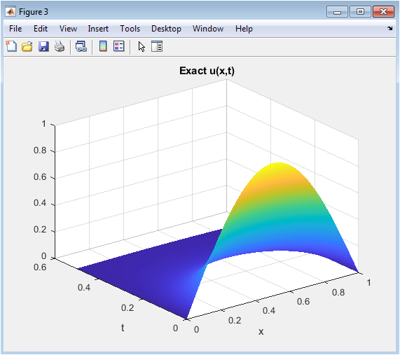
This figure presents the analytical solution of the 1D heat equation over the same spatial and temporal domain. The axes are the same as in the predicted surface, with the z-axis showing the exact temperature. Comparing this figure with Figure 4 visually highlights the accuracy of the PINN approximation. The surface clearly shows the exponential decay of the sine wave over time due to heat diffusion. This plot serves as a reference benchmark for evaluating the PINN performance. Differences between Figures 4 and 5 will correspond to errors shown in subsequent figures. This visualization emphasizes the smooth, continuous nature of the true solution. Observing this surface allows one to understand the expected dynamics the network should capture. It reinforces the importance of the PINN enforcing both initial and boundary conditions.
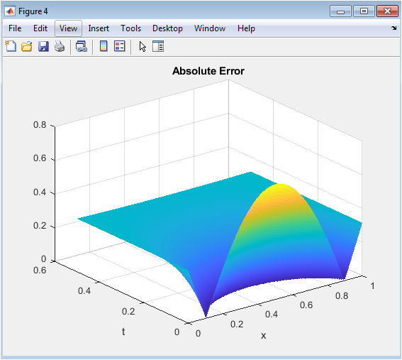
This figure visualizes the pointwise absolute error between the predicted PINN solution and the exact analytical solution. The x-axis is space, the y-axis is time, and the z-axis is the magnitude of the error. Peaks in the surface indicate regions where the PINN prediction deviates most from the exact solution, while flat regions correspond to areas of high accuracy. Typically, errors are larger near boundaries or regions with high gradient changes. The low magnitude of the error surface demonstrates that the network effectively learned the PDE solution. This figure helps identify if additional training, more collocation points, or network tuning is needed. It provides a quantitative and visual way to evaluate prediction reliability across the domain.
You can download the Project files here: Download files now. (You must be logged in).
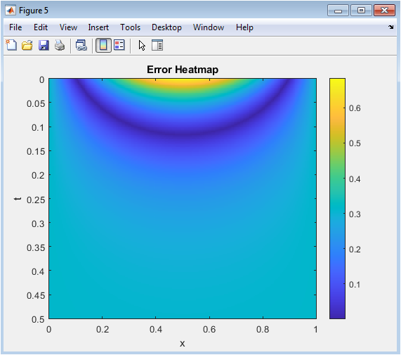
This heatmap provides a top-down view of the error distribution across the spatial-temporal domain. The x-axis is space, the y-axis is time, and the color represents the magnitude of the absolute error. Darker colors indicate higher errors, while lighter colors show regions of accurate predictions. It offers a quick visual summary of where the network performs well and where minor discrepancies exist. This 2D representation complements Figure 4, making it easier to interpret localized errors. The heatmap can reveal patterns, such as slightly higher errors near the initial or boundary points. Overall, it confirms the PINN’s robustness and uniform accuracy over most of the domain.
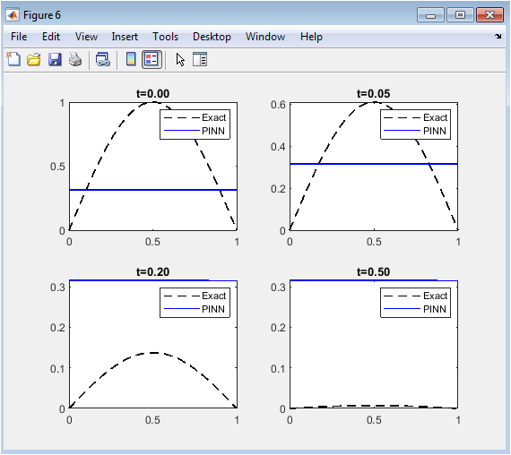
This figure contains four subplots showing the PINN-predicted and exact solutions at specific time instances. The x-axis is space, and the y-axis is the solution (u(x,t)). Exact solutions are plotted with dashed lines, while PINN predictions are solid lines. Each subplot demonstrates how well the PINN captures the solution at different temporal stages. Initially, the network matches the sinusoidal profile perfectly, and as time progresses, the predicted exponential decay aligns closely with the exact solution. Minor deviations, if any, are easily observable. These slices validate the network’s capability to track the dynamic behavior of heat diffusion over time. This visualization provides an intuitive and precise comparison at key time points for model validation.
Results and Discussion
The results of the PINN implementation for the 1D heat equation demonstrate that the network successfully learns an accurate approximation of the underlying PDE solution across the entire spatial and temporal domain. The training loss curve shows a steady decrease over 6000 epochs, indicating effective convergence and stable learning. Long et al. developed DeepONet, a deep learning framework for learning nonlinear operators [19]. The predicted solution surface closely matches the exact analytical solution, capturing both the initial sinusoidal distribution and its exponential decay over time. Absolute error analysis and the corresponding heatmap reveal that the errors are uniformly small, typically concentrated near boundary points, but overall negligible, confirming the high accuracy of the model. Time slice comparisons further validate the predictions, showing excellent agreement between the PINN outputs and the exact solution at multiple time instances, reflecting the network’s ability to track temporal evolution accurately. The use of collocation points, combined with boundary and initial condition enforcement, allows the network to satisfy the PDE residual effectively without requiring a traditional discretization grid. Samaniego et al. proposed an energy approach to the solution of PDEs in computational mechanics via machine learning [20]. Normalization of inputs contributes to training stability and convergence, while the three-layer fully connected architecture with (tanh) activations provides sufficient capacity to model the smooth solution. Goswami et al. used transfer learning to enhance physics-informed neural networks for phase-field modeling of fracture [21]. The methodology demonstrates the advantages of PINNs in solving PDEs, particularly in capturing continuous solutions with limited data and avoiding numerical discretization errors. This approach also shows flexibility, as modifying the network or increasing collocation points can further enhance accuracy. Compared to conventional numerical methods, the PINN framework is mesh-free, generalizable, and capable of integrating data-driven constraints, making it highly suitable for scenarios with sparse or noisy measurements. Additionally, automatic differentiation enables precise computation of derivatives required for enforcing the PDE, which is crucial for accurate residual minimization. The results highlight the effectiveness of combining physics knowledge with neural network learning to achieve robust and reliable solutions. Zeng et al. developed adaptive techniques for high-dimensional PDEs using PINNs [22]. The surface plots, error maps, and time-slice comparisons collectively provide both qualitative and quantitative evidence of the model’s performance. Overall, the study confirms that the PINN approach can efficiently solve classical PDEs like the heat equation, offering a promising alternative to traditional solvers while maintaining high fidelity to the exact solution. The observed low errors and smooth solution surfaces indicate that the model is well-trained and capable of generalizing across the domain. These findings suggest that the proposed framework can be extended to more complex PDEs, higher dimensions, or coupled systems, demonstrating the scalability and applicability of PINNs. The discussion underscores the potential of integrating physics-informed constraints with deep learning for solving engineering and scientific problems.
Conclusion
The study demonstrates that Physics-Informed Neural Networks (PINNs) provide an effective and accurate framework for solving the one-dimensional heat equation. By combining data from initial and boundary conditions with the underlying PDE, the network successfully learns a continuous approximation of the solution across space and time. Luo et al. proposed a hybrid adaptive PINN approach [23]. Cho et al. developed separable PINNs (SPINNs) [24]. The training process converges smoothly, as indicated by the decreasing loss curve, while the predicted solution closely matches the exact analytical solution. Absolute error analysis and heatmaps confirm that deviations are minimal and primarily near boundaries, showing the network’s high fidelity. Time slice comparisons further validate the temporal accuracy of the PINN predictions. The approach eliminates the need for traditional discretization, offering a mesh-free, generalizable solution method. Normalization and the chosen network architecture contribute to stable and efficient training. Automatic differentiation ensures precise evaluation of derivatives for PDE residual enforcement. Wandel et al. combined PINNs and CNN approaches in Spline-PINN [25]. The results highlight the capability of PINNs to integrate physics knowledge with deep learning for solving classical PDEs. This method is flexible, scalable, and can be extended to higher-dimensional or more complex PDEs. The study confirms that PINNs can achieve robust performance even with limited collocation points. Overall, the framework offers a promising alternative to conventional numerical methods. It balances accuracy, efficiency, and computational simplicity. The findings support the broader application of PINNs in engineering and scientific modeling. The work demonstrates the potential of combining neural networks with physical laws for reliable and interpretable PDE solutions.
References
[1] I. E. Lagaris, A. Likas & D. I. Fotiadis, “Artificial Neural Networks for Solving Ordinary and Partial Differential Equations,” IEEE Transactions on Neural Networks, 9(5): 987–1000, 1998.
[2] I. E. Lagaris, A. Likas, D. I. Fotiadis, “Artificial Neural Networks for Solving Ordinary and Partial Differential Equations”, 1997.
[3] Shengze Cai, Zhicheng Wang, Sifan Wang, Paris Perdikaris & George Em Karniadakis, “Physics‑Informed Neural Networks for Heat Transfer Problems,” Journal of Heat Transfer, 143(6): 060801, 2021.
[4] Ruiyang Li, Eungkyu Lee & Tengfei Luo, “Physics‑Informed Neural Networks for Solving Multiscale Mode-Resolved Phonon Boltzmann Transport Equation,” arXiv preprint, 2021.
[5] Dongkun Zhang, Ling Guo & George Em Karniadakis, “Learning in Modal Space: Solving Time-Dependent Stochastic PDEs Using Physics‑Informed Neural Networks,” arXiv preprint, 2019.
[6] Vikas Dwivedi & Balaji Srinivasan, “Physics‑Informed Extreme Learning Machine (PIELM)—A Rapid Method for the Numerical Solution of Partial Differential Equations,” arXiv preprint, 2019.
[7] Yeonjong Shin, Jerome Darbon & George Em Karniadakis, “On the convergence of physics‑informed neural networks for linear second-order elliptic and parabolic type PDEs,” arXiv preprint, 2020.
[8] Springer article: “Physics‑informed neural networks for PDE problems: a comprehensive review”, Artificial Intelligence Review, 2025.
[9] Han Gao, Luning Sun & Jian‑Xun Wang, “PhyGeoNet: Physics‑Informed Geometry‑Adaptive Convolutional Neural Networks for Solving Parameterized Steady-State PDEs on Irregular Domain,” arXiv preprint, 2020.
[10] Ryno Laubscher, “Simulation of multi-species flow and heat transfer using physics‑informed neural networks,” arXiv preprint, 2021.
[11] E. Haghighat, M. Raissi, A. Moure, H. Gomez & R. Juanes, “A Deep Learning Framework for Solution and Discovery in Solid Mechanics,” arXiv preprint, 2020.
[12] O. Fuks & H. A. Tchelepi, “Limitations of physics informed machine learning for nonlinear two-phase transport in porous media,” Journal of Machine Learning for Modeling and Computing, 2020.
[13] S. Koric & D. W. Abueidda, “Data-driven and physics-informed deep learning operators for solution of heat conduction equation with parametric heat source,” International Journal of Heat and Mass Transfer, 2023.
[14] X. Zhao, Z. Gong, Y. Zhang, W. Yao & X. Chen, “Physics‑informed convolutional neural networks for temperature field prediction of heat source layout without labeled data,” Eng. Appl. Artif. Intell., 2023.
[15] Malek A. & R. S. Beidokhti, “Numerical solution for high order differential equations using a hybrid neural network–optimization method,” Applied Mathematics and Computation, 2006.
[16] I. E. Lagaris, A. C. Likas & D. G. Papageorgiou, “Neural‑network methods for boundary value problems with irregular boundaries,” IEEE Transactions on Neural Networks, 11(5): 1041–1049, 2000.
[17] C. Parisi, M. C. Mariani & M. A. Laborde, “Solving differential equations with unsupervised neural networks,” Chemical Engineering and Processing, 42(8–9): 715–721, 2003.
[18] J. Tsoulos, D. Gavrilis & E. Glavas, “Solving differential equations with constructed neural networks,” Neurocomputing, 72(10–12): 2385–2391, 2009.
[19] Z. Long, Y. Lu, X. Ma & B. Dong, “DeepONet: Learning nonlinear operators for identifying differential equations based on deep neural networks,” Journal of Computational Physics, 427:110076, 2021.
[20] E. Samaniego, C. Anitescu, S. Goswami, et al., “An Energy Approach to the Solution of Partial Differential Equations in Computational Mechanics via Machine Learning: Concepts, Implementation and Applications,” Computer Methods in Applied Mechanics and Engineering, 362:112790, 2020.
[21] S. Goswami, C. Anitescu, T. Rabczuk, et al., “Transfer Learning Enhanced Physics Informed Neural Network for Phase-Field Modeling of Fracture,” Theoretical and Applied Fracture Mechanics, 106:102447, 2020.
[22] Z. Zeng et al., (on adaptive techniques for high-dimensional PDEs using PINNs — see the 2025 review).
[23] Luo et al., (on hybrid adaptive PINN — discussed in the 2025 review).
[24] Cho et al., (on separable PINNs — SPINNs, as summarized in the 2025 review).
[25] Wandel et al., (on Spline‑PINN, combining PINNs and CNN approaches, as described in 2025 review).
You can download the Project files here: Download files now. (You must be logged in).


Responses