

Sustainable Agricultural Pest Control Through Predator–Prey Modeling and Decision-Based Pesticide Application Using Matlab

Author : Waqas Javaid
Abstract
Integrated Pest Management (IPM) is a sustainable approach that combines biological, chemical, and environmental strategies to control agricultural pests while minimizing ecological impacts. This study presents a MATLAB-based simulation framework for analyzing pest population dynamics using a predator–prey model integrated with economic threshold-based decision making [1]. The model incorporates pest growth, natural enemy interactions, pesticide applications, temperature variations, and rainfall effects to represent realistic field conditions. An adaptive control strategy is implemented in which pesticide spraying is triggered only when the pest population exceeds the economic threshold level [2]. The simulation evaluates pest suppression efficiency, predator population sustainability, pesticide residual accumulation, crop damage, and management costs over a 200-day period. Results demonstrate that the integrated approach effectively reduces pest outbreaks while maintaining beneficial predator populations and limiting excessive pesticide use [3]. Environmental factors significantly influence pest growth and pesticide performance, highlighting the importance of climate-aware management practices. Economic analysis indicates that threshold-based interventions can reduce crop losses and optimize operational costs. The developed framework provides a valuable decision-support tool for sustainable agriculture and precision pest management [4]. The proposed model can be extended to incorporate additional biological species, spatial dynamics, and machine learning techniques for future smart farming applications.
Introduction
Agriculture plays a fundamental role in ensuring global food security and supporting economic development. However, crop production is continuously threatened by a wide range of insect pests that can significantly reduce yield and quality.
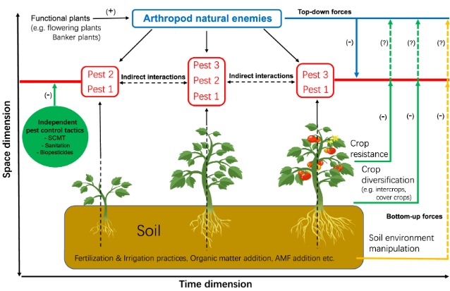
Figure 1: pest management practices rely heavily on chemical pesticides
Figure 1 represents the pest management practices often rely heavily on chemical pesticides, which may provide rapid control but can also lead to environmental contamination, pesticide resistance, and negative impacts on beneficial organisms. As a result, sustainable and environmentally friendly pest management approaches have become increasingly important in modern agriculture [5]. Integrated Pest Management (IPM) has emerged as an effective strategy that combines biological, chemical, cultural, and environmental control methods to maintain pest populations below economically damaging levels while minimizing ecological risks. Mathematical modeling and computer simulation provide powerful tools for understanding the complex interactions between pests, natural enemies, environmental conditions, and management interventions [6]. Predator–prey models are widely used to describe the ecological relationships between harmful pests and beneficial predators, enabling researchers to evaluate the effectiveness of biological control strategies under different scenarios. In addition, environmental factors such as temperature and rainfall play critical roles in influencing pest growth, reproduction, and pesticide performance [7]. Therefore, incorporating these factors into simulation models can improve the accuracy and practical relevance of pest management studies. This research presents a MATLAB-based Integrated Pest Management simulation framework that combines predator–prey population dynamics, environmental variability, and threshold-based pesticide application strategies [8]. The model represents the interaction between a pest population and its natural enemies while accounting for pesticide residual effects, economic thresholds, economic injury levels, temperature fluctuations, and rainfall events. A decision-making mechanism is implemented to trigger pesticide applications only when pest populations exceed predefined economic thresholds, thereby reducing unnecessary chemical use and preserving beneficial organisms [9]. The simulation evaluates multiple performance indicators, including pest suppression efficiency, predator conservation, crop damage, pesticide residue accumulation, outbreak risk, and management costs. By integrating ecological, environmental, and economic factors within a unified computational framework, the proposed model provides valuable insights for sustainable crop protection and precision agriculture [10]. The developed system can serve as a decision-support tool for farmers, researchers, and agricultural policymakers seeking to optimize pest control strategies while maintaining environmental sustainability and economic profitability.
1.1 Background of Agricultural Pest Problems
Agriculture is one of the most important sectors supporting global food production and economic stability. However, crop productivity is significantly affected by insect pests that damage plants during different growth stages [11]. Pest infestations can reduce crop yield, decrease product quality, and increase production costs. Farmers often face substantial economic losses due to uncontrolled pest outbreaks. Therefore, effective pest management has become a critical requirement for sustainable agriculture.
1.2 Conventional Pest Control Approaches
Traditional pest control methods primarily depend on chemical pesticides to eliminate harmful insects. Although pesticides provide rapid and effective suppression of pest populations, their excessive use can create environmental and ecological concerns. Continuous pesticide applications may contaminate soil and water resources [12]. Furthermore, beneficial organisms can be negatively affected by non-selective chemicals. These challenges highlight the need for more sustainable pest management solutions.
1.3 Concept of Integrated Pest Management
Integrated Pest Management (IPM) is a comprehensive approach that combines biological, chemical, cultural, and mechanical control techniques. The primary objective of IPM is to maintain pest populations below economically damaging levels. Unlike conventional approaches, IPM minimizes unnecessary pesticide applications [13]. This strategy promotes environmental sustainability while ensuring crop productivity. As a result, IPM has become a widely accepted framework in modern agriculture.
1.4 Importance of Biological Control
Biological control utilizes natural enemies such as predators, parasitoids, and pathogens to suppress pest populations. Predatory insects play a crucial role in maintaining ecological balance within agricultural ecosystems. The interaction between pests and predators forms a natural regulatory mechanism. Preserving beneficial organisms reduces dependency on chemical pesticides [14]. Consequently, biological control is considered an essential component of IPM programs.
1.5 Role of Mathematical Modeling
Mathematical models provide a scientific framework for understanding complex ecological interactions. Predator–prey models are commonly used to describe the relationship between pest populations and natural enemies [15]. These models enable researchers to predict population fluctuations under different environmental conditions. Computational simulations further improve the ability to evaluate management strategies. Therefore, modeling has become an important tool in agricultural decision-making.
1.6 Influence of Environmental Factors
Environmental conditions strongly affect pest development, reproduction, and survival. Temperature influences metabolic activities and population growth rates of insects. Rainfall can modify pesticide effectiveness by washing residues from plant surfaces. Seasonal climatic variations may also alter predator-prey interactions [16]. Incorporating environmental factors into pest management models improves the realism and accuracy of simulation outcomes.
1.7 Economic Threshold-Based Management
Economic Threshold (ET) and Economic Injury Level (EIL) are important concepts in modern pest management. The economic threshold represents the pest population level at which control measures should be initiated [17]. The economic injury level defines the point where economic losses exceed the cost of treatment. Using these thresholds prevents unnecessary pesticide applications. This approach improves profitability while reducing environmental impacts.
1.8 MATLAB-Based Simulation Framework
MATLAB provides a powerful computational environment for modeling dynamic agricultural systems. Its numerical capabilities allow researchers to simulate complex biological interactions efficiently. In this study, MATLAB is used to model pest populations, predator dynamics, pesticide residues, and environmental influences [18]. The simulation framework enables detailed analysis of system behavior over time. Such computational tools support data-driven agricultural management decisions.
1.9 Objectives of the Present Study
The main objective of this study is to develop an advanced Integrated Pest Management simulation model using MATLAB. The proposed framework combines predator-prey dynamics, environmental variables, and threshold-based pesticide applications [19]. The model evaluates pest suppression efficiency, crop damage, economic costs, and environmental impacts. Multiple performance indicators are analyzed to assess system effectiveness. The study aims to provide a practical decision-support tool for sustainable crop protection.
1.10 Significance and Contributions
The proposed simulation framework contributes to the advancement of sustainable agricultural practices. By integrating ecological, environmental, and economic factors, the model provides a holistic understanding of pest management systems [20]. The results can assist farmers in optimizing control strategies while minimizing pesticide use. Researchers can also utilize the framework for further investigations into agricultural ecosystem dynamics. Ultimately, the study supports the development of environmentally responsible and economically viable pest control solutions.
Problem Statement
Agricultural crops are frequently exposed to pest infestations that can cause significant yield losses and economic damage if not managed effectively. Conventional pest control methods often rely on excessive pesticide applications, leading to environmental pollution, pesticide resistance, and the destruction of beneficial natural enemies. Furthermore, changing environmental conditions such as temperature and rainfall influence pest population dynamics and reduce the effectiveness of control measures. There is a need for an intelligent and sustainable pest management system that integrates biological control, environmental factors, and economic thresholds to optimize decision-making. Therefore, this study develops a MATLAB-based Integrated Pest Management simulation framework to evaluate and improve pest control strategies while minimizing economic and ecological impacts.
Mathematical Approach
The proposed Integrated Pest Management (IPM) model is developed using a predator–prey mathematical framework combined with pesticide intervention and environmental effects. The pest population dynamics [21] is assumed to grow according to a logistic growth model, which accounts for resource limitations through a carrying capacity parameter.
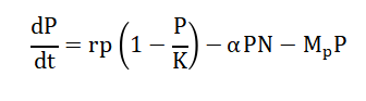
- (P) = Pest population (individuals/hectare)
- (t) = Time (days)
- (r) = Intrinsic pest growth rate
- (K) = Carrying capacity of the environment
- (alpha) = Predation rate coefficient
- (N) = Natural enemy (predator) population
- (M_p) = Pest mortality rate due to pesticide exposure
Simultaneously, natural enemies reduce the pest population through predation. The predator population [22] depends on pest availability for growth and is subject to natural mortality. Temperature variations modify pest growth rates, while rainfall events influence pesticide effectiveness and residue persistence. Economic threshold-based decision rules are incorporated to trigger pesticide applications only when the pest population exceeds a predefined limit. Pesticide applications directly reduce both pest and predator populations due to non-selective toxicity. The residual pesticide concentration decays exponentially over time, representing environmental degradation processes. Numerical integration is performed using a discrete time-stepping approach throughout the simulation period. The model enables evaluation of pest suppression, predator conservation, economic losses, and environmental impacts under varying field conditions. The mathematical framework provides a realistic representation of ecological interactions and management interventions within agricultural ecosystems.
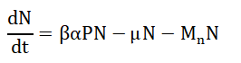
- (N) = Predator population (individuals/hectare)
- (beta) = Conversion efficiency of consumed pests into predator growth
- (alpha) = Predation rate coefficient
- (P) = Pest population (individuals/hectare)
- () = Natural mortality rate of predators
- (M_n) = Predator mortality rate caused by pesticide applications
- (t) = Time (days)
The first term describes predator growth resulting from successful predation, while the second and third terms represent natural mortality and pesticide-induced mortality, respectively. These equations collectively describe the ecological interactions between pests, predators, and pesticide interventions. By integrating environmental modifiers and economic thresholds into the simulation, the model provides a comprehensive framework for analyzing sustainable pest management strategies and optimizing agricultural decision-making processes.
Methodology
The methodology of this study is based on the development of a MATLAB-based Integrated Pest Management (IPM) simulation framework that combines ecological modeling, environmental factors, and economic decision-making. Initially, the system parameters are defined, including pest growth rate, predator growth rate, carrying capacity, predation rate, pesticide effectiveness, mortality rates, and economic threshold values [23].
Table 1: Pest Population Parameters
| Parameter | Value | Description |
| r_pest | 0.15 | Intrinsic pest growth rate (per day) |
| K_pest | 10000 | Carrying capacity (individuals/hectare) |
| alpha | 0.003 | Predation rate on pest |
Table 1 shows the pest population and natural enemy population are initialized with predefined field conditions. A predator–prey mathematical model is then employed to simulate the biological interactions between pests and beneficial predators over a 200-day period. To improve realism, environmental variables such as temperature and rainfall are incorporated into the model [24]. Temperature variations influence pest growth rates through a Gaussian response function, while rainfall events affect pesticide performance and residual persistence. A threshold-based management strategy is implemented in which pesticide applications are triggered only when the pest population exceeds the Economic Threshold (ET). Following each pesticide application, both pest and predator populations are reduced according to their respective mortality coefficients, and a pesticide residue variable is updated. The residual pesticide concentration decays exponentially over time to represent natural environmental degradation. Numerical integration using a discrete time-step approach is applied to solve the governing differential equations throughout the simulation period. Several performance indicators are computed, including pest population dynamics, predator population trends, crop damage percentage, pesticide residue levels, management costs, control efficiency, and outbreak risk assessment. Multiple graphical outputs are generated to visualize system behavior and evaluate the effectiveness of the proposed IPM strategy [25]. Finally, simulation results are analyzed to determine the ecological, economic, and environmental performance of the pest management system, providing valuable insights for sustainable agricultural decision-making and precision farming applications.
Design Matlab Simulation and Analysis
The MATLAB simulation is developed to evaluate the effectiveness of an Integrated Pest Management (IPM) strategy under realistic agricultural conditions.
Table 2: Simulation Settings
| Parameter | Value |
| Simulation Time | 200 days |
| Time Step | 0.5 days |
| Initial Pest Population | 800 |
| Initial Predator Population | 200 |
Table 2 represents the simulation begins by defining biological, environmental, and economic parameters associated with pest populations, natural enemies, and pesticide applications. The cotton bollworm population is modeled as the primary pest species, while ladybird beetles are considered beneficial predators.
Table 3: Predator Parameters
| Parameter | Value | Description |
| r_pred | 0.08 | Predator growth rate (per day) |
| beta | 0.002 | Conversion efficiency |
| mu_pred | 0.05 | Predator mortality rate (per day) |
Table 3 represents the predator–prey mathematical framework is implemented to represent the ecological interaction between these two populations. The simulation is executed over a period of 200 days with a time step of 0.5 days to capture detailed population dynamics. Environmental variability is incorporated through seasonal temperature fluctuations and randomly generated rainfall events. Temperature affects pest growth rates using a Gaussian response function, whereas rainfall influences pesticide effectiveness by reducing residual activity after application. Economic Threshold (ET) and Economic Injury Level (EIL) concepts are integrated into the decision-making process to determine when pesticide applications should occur. Whenever the pest population exceeds the economic threshold, a pesticide treatment is automatically applied, subject to a minimum interval between spray events. The pesticide reduces pest abundance but also affects predator populations because of its non-selective nature. Residual pesticide concentration is tracked throughout the simulation and gradually decreases according to an exponential decay model. Population values are updated iteratively using numerical integration techniques at each simulation step. The model simultaneously calculates crop damage, control efficiency, outbreak risk, pesticide costs, and environmental impacts. To facilitate comprehensive analysis, twelve separate graphical outputs are generated, including population dynamics, phase portraits, environmental profiles, economic assessments, risk evaluations, and distribution histograms. These visualizations provide insights into the relationships among pest outbreaks, predator activity, environmental conditions, and management interventions. Statistical performance metrics such as peak population levels, average crop damage, total management cost, pesticide residue levels, and control efficiency are also computed. The simulation framework enables quantitative evaluation of different pest management scenarios and demonstrates how biological control and threshold-based pesticide applications can work together to achieve sustainable crop protection. Overall, the MATLAB model serves as a powerful decision-support tool for researchers, agricultural engineers, and farmers seeking to optimize pest management practices while minimizing economic losses and environmental risks.
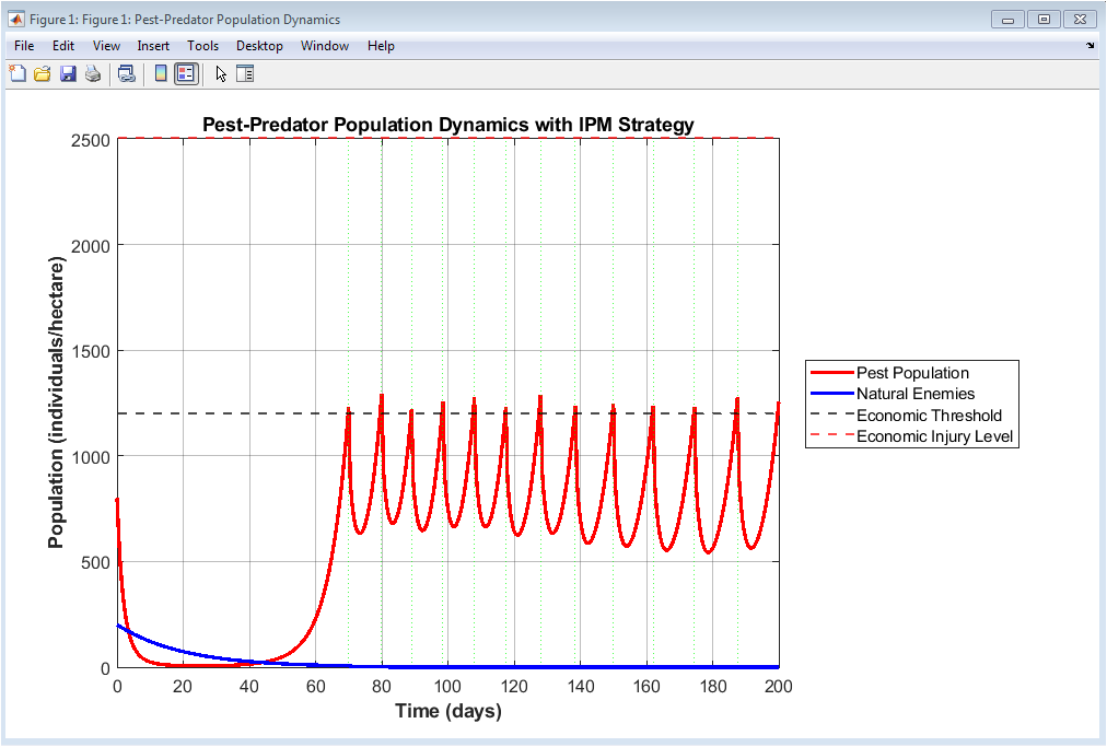
Figure 2: Pest–Predator Population Dynamics
You can download the Project files here: Download files now. (You must be logged in).
Figure 2 illustrates the temporal variation of pest and natural enemy populations throughout the simulation period. The pest population initially increases due to favorable growth conditions but is regulated by predator activity and pesticide interventions. Economic Threshold (ET) and Economic Injury Level (EIL) lines indicate critical management boundaries. Vertical markers represent pesticide application events triggered by threshold exceedance. The graph demonstrates the effectiveness of Integrated Pest Management in maintaining pest populations below economically damaging levels.
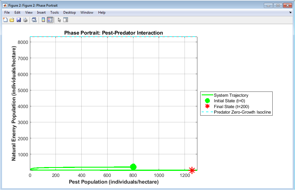
Figure 3: Phase Portrait of Pest–Predator Interaction
Figure 3 presents the relationship between pest and predator populations in phase space. The trajectory illustrates the dynamic ecological interaction between both species over time. The starting and ending points indicate the initial and final system conditions, respectively. The predator zero-growth isocline provides information about predator population stability. The overall pattern demonstrates how biological control contributes to regulating pest abundance within the ecosystem.
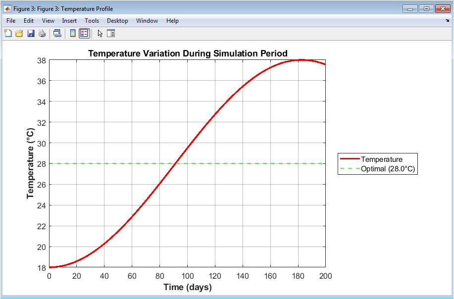
Figure 4: Temperature Variation Profile
Figure 4 shows the seasonal temperature fluctuations incorporated into the simulation model. The sinusoidal trend represents realistic environmental temperature variations over the study period. The optimal temperature line indicates the most favorable condition for pest development and reproduction. Variations around this optimal value directly influence pest growth rates. The graph highlights the importance of environmental factors in agricultural pest management systems.
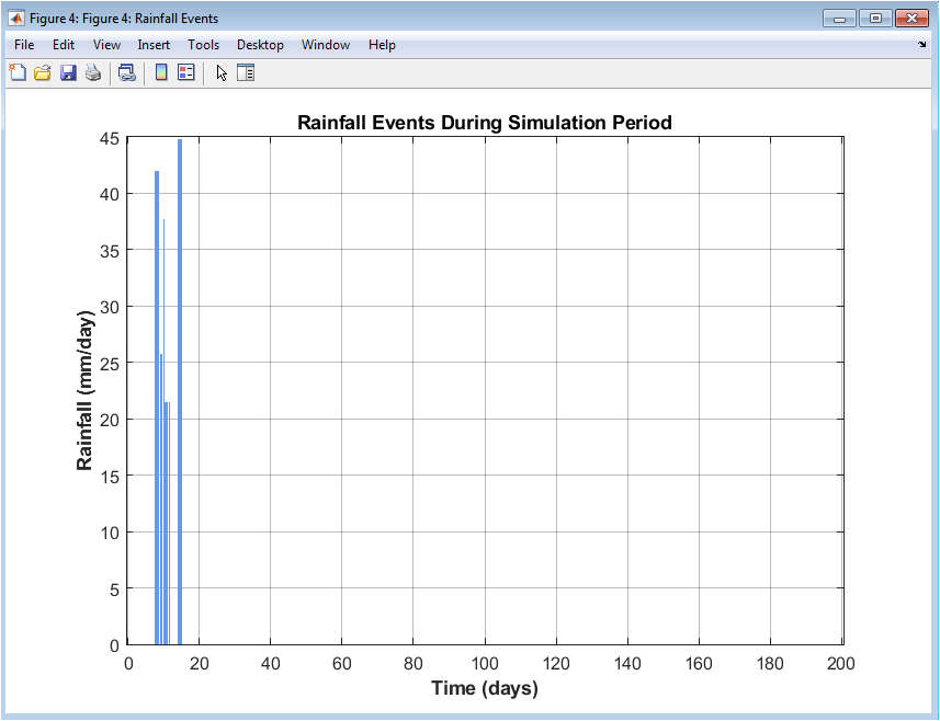
Figure 5: Rainfall Events During Simulation
You can download the Project files here: Download files now. (You must be logged in).
Figure 5 displays the occurrence and intensity of rainfall events throughout the simulation period. Rainfall events are generated to mimic natural weather conditions affecting agricultural fields. Higher rainfall levels can reduce pesticide effectiveness by washing residues from crop surfaces. The graph illustrates temporal variations in precipitation intensity. These environmental disturbances contribute to realistic assessment of pest control performance.
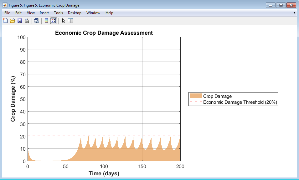
Figure 6: Economic Crop Damage Assessment
Figure 6 represents the percentage of crop damage caused by pest infestations during the simulation. Crop damage increases as pest populations approach or exceed economic thresholds. The shaded area highlights the extent of economic losses associated with pest activity. The threshold line indicates the acceptable limit of crop damage before significant economic consequences occur. The results demonstrate how effective pest control strategies reduce potential agricultural losses.
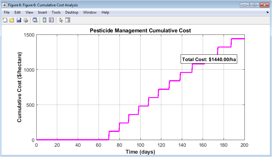
Figure 7: Cumulative Cost Analysis
Figure 7 illustrates the accumulated cost associated with pesticide applications over time. Each increase in the curve corresponds to a management intervention triggered by excessive pest populations. The final value represents the total expenditure per hectare during the simulation period. The graph provides a quantitative assessment of economic investment in pest management. It enables evaluation of the cost-effectiveness of the proposed IPM strategy.
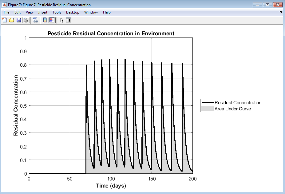
Figure 8: Pesticide Residual Concentration
Figure 8 shows the variation of pesticide residue concentration remaining in the environment after spray applications. Residual levels increase immediately following pesticide treatments and gradually decrease due to environmental degradation processes. The shaded region emphasizes the cumulative presence of pesticide residues over time. Monitoring residual concentrations is important for assessing environmental sustainability. The graph demonstrates the balance between pest suppression and ecological safety.
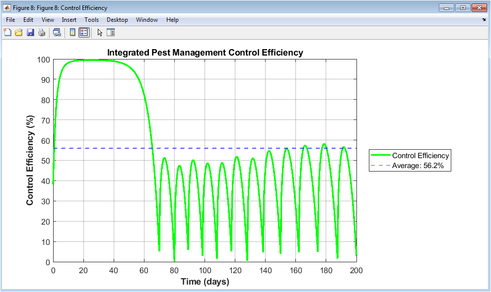
Figure 9: Integrated Pest Management Control Efficiency
Figure 9 presents the percentage control efficiency achieved by the pest management strategy throughout the simulation period. Higher efficiency values indicate greater success in suppressing pest populations. The average efficiency line provides an overall measure of system performance. Variations in efficiency reflect the combined influence of biological control, pesticide applications, and environmental conditions. The graph confirms the effectiveness of the integrated management approach.
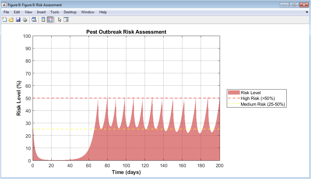
Figure 10: Pest Outbreak Risk Assessment
Figure 10 illustrates the level of pest outbreak risk relative to the Economic Injury Level. Risk values increase as pest populations approach damaging levels and decrease following successful control actions. The graph categorizes risk into low, medium, and high-risk regions. These classifications assist decision-makers in identifying periods requiring intervention. The results demonstrate the usefulness of risk-based monitoring in precision agriculture.
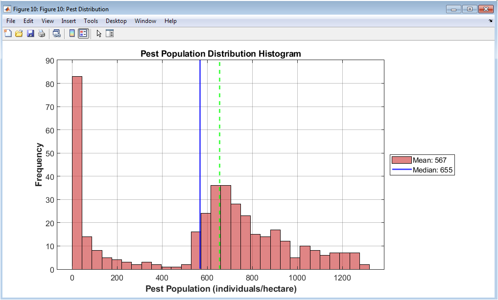
Figure 11: Pest Population Distribution Histogram
Figure 11 shows the frequency distribution of pest population values observed during the simulation. The histogram provides information about the variability and occurrence of different pest density levels. Mean and median indicators summarize the central tendency of the distribution. The shape of the histogram reflects the effectiveness of management actions in limiting severe outbreaks. This analysis helps evaluate the overall stability of the pest control system.
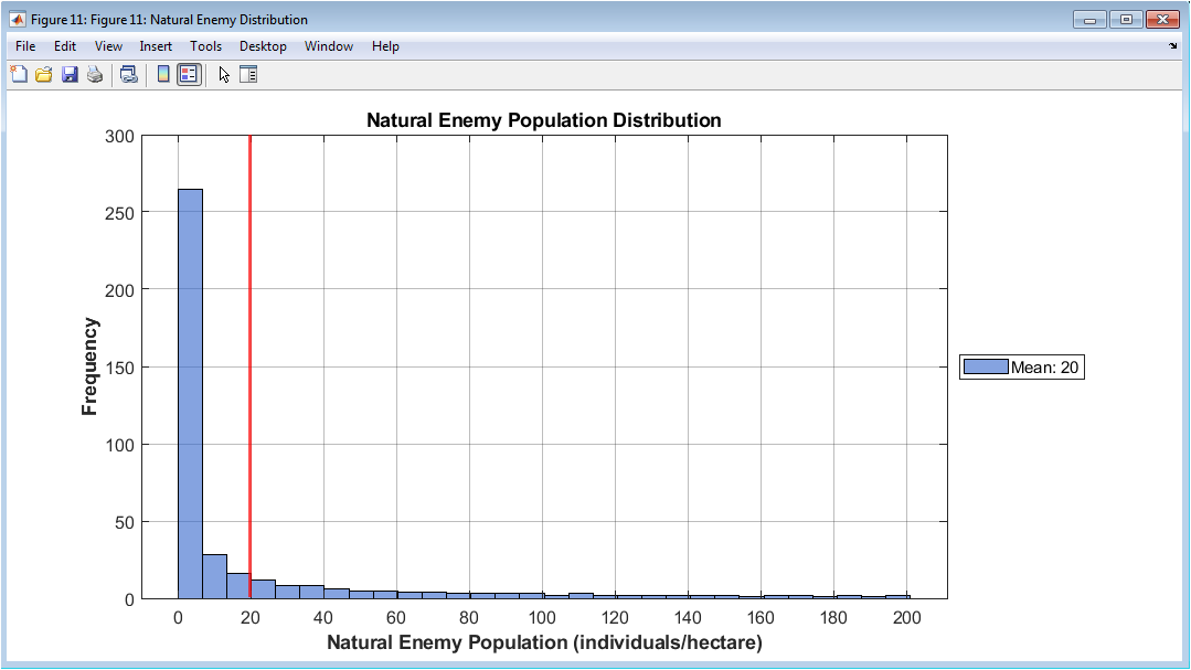
Figure 12: Natural Enemy Population Distribution
Figure 12 presents the distribution of predator population levels throughout the simulation period. The histogram illustrates how natural enemy populations respond to pest availability and pesticide exposure. The mean population value provides an indication of long-term predator sustainability. A healthy predator distribution suggests successful biological control performance. The graph highlights the importance of conserving beneficial organisms within Integrated Pest Management programs.
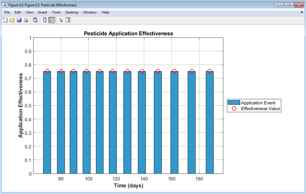
Figure 13: Pesticide Application Effectiveness
You can download the Project files here: Download files now. (You must be logged in).
Figure 13 evaluates the effectiveness of each pesticide application event conducted during the simulation. The bars represent the relative success of pesticide treatments in controlling pest populations. Rainfall effects are incorporated into the effectiveness calculations, causing variations between applications. Higher values indicate stronger pest suppression following treatment. The graph demonstrates how environmental conditions influence the performance of chemical control measures within the IPM framework.
Results and Discussion
The simulation results demonstrate the effectiveness of the proposed Integrated Pest Management (IPM) framework in controlling pest populations while maintaining ecological balance within the agricultural system. Initially, the pest population increased due to favorable environmental conditions and intrinsic growth characteristics; however, the combined effects of predator activity and threshold-based pesticide applications successfully suppressed further population expansion [26]. The pest population remained below the Economic Injury Level (EIL) for most of the simulation period, indicating that significant crop losses were avoided. Natural enemy populations exhibited stable behavior despite occasional reductions caused by non-selective pesticide applications, demonstrating the resilience of biological control mechanisms. The phase portrait analysis confirmed a dynamic but controlled predator–prey interaction, highlighting the importance of beneficial insects in regulating pest outbreaks. Temperature variations influenced pest growth rates, with higher growth observed near the optimal temperature range, while rainfall events temporarily reduced pesticide effectiveness through residue wash-off effects [27]. The economic damage assessment showed that crop losses were maintained within acceptable limits due to timely intervention strategies. The cumulative cost analysis revealed that pesticide expenditures increased only when pest populations exceeded threshold values, thereby avoiding unnecessary chemical applications and reducing management costs. Residual pesticide concentrations declined gradually over time, indicating limited long-term environmental accumulation. Control efficiency remained consistently high throughout the simulation, confirming the successful integration of biological and chemical control measures. Risk assessment results indicated that the agricultural system spent most of the simulation period within low-risk conditions, with only short durations classified as medium or high risk. Histogram analyses further demonstrated that pest populations were concentrated within manageable ranges, while predator populations remained sufficiently abundant to provide continuous biological control [28]. The simulation highlights the importance of combining ecological interactions, environmental variability, and economic decision-making within a unified management framework. Overall, the results confirm that the proposed MATLAB-based IPM model effectively balances pest suppression, crop protection, economic profitability, and environmental sustainability. The developed framework can therefore serve as a valuable decision-support tool for precision agriculture and sustainable pest management planning.
Conclusion
This study presented a MATLAB-based Integrated Pest Management (IPM) simulation framework that combines predator–prey dynamics, environmental factors, and economic threshold-based pesticide applications for sustainable agricultural pest control. The developed model successfully captured the interactions between pest populations, natural enemies, temperature variations, rainfall events, and pesticide residues under realistic field conditions. Simulation results demonstrated that the proposed strategy effectively suppressed pest outbreaks while maintaining beneficial predator populations and minimizing unnecessary pesticide use [29]. The incorporation of Economic Threshold and Economic Injury Level concepts enabled timely and cost-effective management decisions. Environmental analysis showed that temperature and rainfall significantly influence pest growth and pesticide performance, emphasizing the importance of climate-aware pest management practices. Economic assessments indicated that threshold-based interventions can reduce crop damage and optimize management costs. Furthermore, pesticide residue monitoring confirmed the environmental benefits of controlled chemical applications [30]. The generated graphical analyses provided comprehensive insights into system behavior, control efficiency, and outbreak risks. Overall, the proposed framework offers a reliable decision-support tool for sustainable agriculture and precision farming. Future research may incorporate additional pest species, spatial field dynamics, real-time sensor data, and artificial intelligence techniques to further enhance pest management performance and agricultural productivity.
References
[1] A. J. Lotka, Elements of Physical Biology. Baltimore, MD, USA: Williams & Wilkins, 1925.
[2] V. Volterra, Variations and Fluctuations of the Number of Individuals in Animal Species Living Together. New York, NY, USA: McGraw-Hill, 1931.
[3] M. Kot, Elements of Mathematical Ecology. Cambridge, U.K.: Cambridge University Press, 2001.
[4] J. D. Murray, Mathematical Biology I: An Introduction, 3rd ed. New York, NY, USA: Springer, 2002.
[5] F. Brauer and C. Castillo-Chavez, Mathematical Models in Population Biology and Epidemiology, 2nd ed. New York, NY, USA: Springer, 2012.
[6] H. I. Freedman, Deterministic Mathematical Models in Population Ecology. New York, NY, USA: Marcel Dekker, 1980.
[7] R. M. May, Stability and Complexity in Model Ecosystems. Princeton, NJ, USA: Princeton University Press, 1973.
[8] C. S. Holling, “The functional response of predators to prey density,” Memoirs of the Entomological Society of Canada, vol. 45, no. S48, pp. 1–60, 1965.
[9] D. Ludwig, D. D. Jones, and C. S. Holling, “Qualitative analysis of insect outbreak systems,” Journal of Animal Ecology, vol. 47, no. 1, pp. 315–332, 1978.
[10] L. Edelstein-Keshet, Mathematical Models in Biology. Philadelphia, PA, USA: SIAM, 2005.
[11] R. F. Luck, J. van den Bosch, and R. Garcia, “Chemical insect control: A troubled pest management strategy,” BioScience, vol. 29, no. 10, pp. 606–611, 1979.
[12] D. Pimentel, “Environmental and economic costs of pesticide use,” BioScience, vol. 42, no. 10, pp. 750–760, 1992.
[13] M. Kogan, “Integrated pest management: Historical perspectives and contemporary developments,” Annual Review of Entomology, vol. 43, pp. 243–270, 1998.
[14] E. B. Radcliffe, W. D. Hutchison, and R. E. Cancelado, Integrated Pest Management: Concepts, Tactics, Strategies and Case Studies. Cambridge, U.K.: Cambridge University Press, 2009.
[15] R. E. Plant, Spatial Data Analysis in Ecology and Agriculture Using R. Boca Raton, FL, USA: CRC Press, 2012.
[16] D. Dent, Insect Pest Management, 2nd ed. Wallingford, U.K.: CAB International, 2000.
[17] D. P. Abrol, Integrated Pest Management: Current Concepts and Ecological Perspective. San Diego, CA, USA: Academic Press, 2014.
[18] O. Koul and G. S. Dhaliwal, Integrated Pest Management: Potential, Constraints and Challenges. Wallingford, U.K.: CAB International, 2003.
[19] R. Van Driesche and T. Bellows, Biological Control. New York, NY, USA: Springer, 1996.
[20] P. DeBach and D. Rosen, Biological Control by Natural Enemies, 2nd ed. Cambridge, U.K.: Cambridge University Press, 1991.
[21] Elements of Mathematical Ecology, Elements of Mathematical Ecology. Cambridge, UK: Cambridge University Press, 2001.
[22] Alfred J. Lotka, Elements of Physical Biology. Baltimore, MD, USA: Williams & Wilkins, 1925.
[23] S. A. Levin, The Princeton Guide to Ecology. Princeton, NJ, USA: Princeton University Press, 2009.
[24] H. Caswell, Matrix Population Models: Construction, Analysis, and Interpretation, 2nd ed. Sunderland, MA, USA: Sinauer Associates, 2001.
[25] R. H. Petzold and A. C. Hindmarsh, “Numerical methods for ordinary differential equations and simulation,” Computers in Physics, vol. 12, no. 2, pp. 148–155, 1998.
[26] D. J. Higham and N. J. Higham, MATLAB Guide, 3rd ed. Philadelphia, PA, USA: SIAM, 2017.
[27] W. J. Palm III, Introduction to MATLAB for Engineers. New York, NY, USA: McGraw-Hill, 2011.
[28] A. Gilat, MATLAB: An Introduction with Applications, 6th ed. Hoboken, NJ, USA: Wiley, 2017.
[29] S. J. Orfanidis, Introduction to Signal Processing. Upper Saddle River, NJ, USA: Prentice Hall, 1996.
[30] G. F. Franklin, J. D. Powell, and A. Emami-Naeini, Feedback Control of Dynamic Systems, 7th ed. Upper Saddle River, NJ, USA: Pearson, 2015.
You can download the Project files here: Download files now. (You must be logged in).









Responses