MATLAB Analysis of a Model Rocket’s Flight Characteristic

Author: Waqas Javaid

Abstract:

This article presents a MATLAB simulation of the flight dynamics of a model rocket. The simulation models the rocket’s trajectory, taking into account the thrust, drag, and gravity forces acting on the rocket. The simulation results provide insights into the rocket’s flight characteristics, including its maximum height, velocity, and acceleration. “The rocket’s propulsion system is a critical component of its overall design [1]. The propulsion system provides the thrust necessary to overcome the force of gravity and propel the rocket into space.” The MATLAB code used in this simulation can be used as a tool for model rocket enthusiasts and researchers to analyze and predict the flight behavior of model rockets.The MATLAB code developed in this study serves as a versatile tool for model rocket enthusiasts, researchers, and educators to analyze and predict the flight behavior of model rockets, facilitating design optimization and performance evaluation. The simulation results demonstrate the effectiveness of MATLAB in modeling and simulating complex dynamic systems, making it an ideal platform for aerospace engineering and physics education.

1.    Introduction:

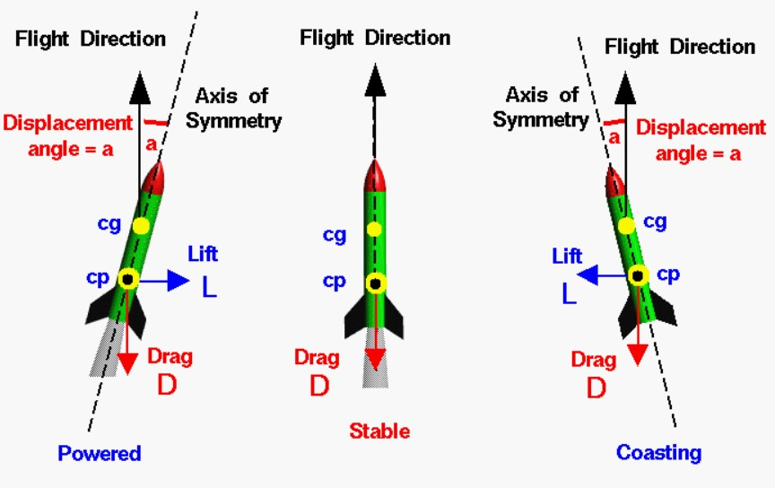
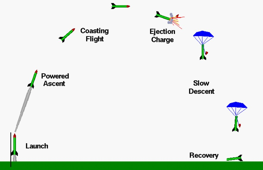
Model rocket’s flight, taking into account the various forces that act upon it. This article can help us understand how the rocket behaves during different phases of its flight, including its ascent, peak altitude, and descent. By analyzing the simulation results, we can gain insights into the rocket’s performance characteristics, such as its maximum height, speed, and acceleration. This type of simulation is not only useful for model rocket enthusiasts but also for educators and researchers looking to study and optimize rocket design and performance.A model rocket’s flight can be broken down into three stages, and throughout these stages, the rocket’s weight remains relatively constant. This is because the amount of fuel burned is negligible compared to the rocket’s overall weight, unlike full-scale rockets which are heavily influenced by their massive fuel loads. During the initial launch phase, the rocket’s thrust far exceeds its weight, allowing it to accelerate rapidly off the launch rail. The aerodynamic forces acting on a rocket, such as lift and drag, play a crucial role in its flight dynamics [2]. Understanding these forces is essential for designing a stable and efficient rocket [3]. The launch rail provides stability at low velocities, preventing the rocket from wobbling or veering off course. As the rocket gains speed, aerodynamic forces come into play, but the thrust remains the dominant force. Once the fuel is depleted, the engine shuts down, and the rocket enters a coasting phase, where it reaches its maximum altitude. At this point, the rocket’s weight and drag forces slow it down, and it begins to fall back towards the ground. As the rocket descends, a delay charge burns, followed by a second charge that deploys the parachute, allowing the rocket to slow down and land safely. The parachute deployment marks the final stage of the rocket’s flight, after which it can be recovered and potentially refurbished for future flights.

2. System Model:

2.1    Launch Phase:

The rocket’s journey begins with a powerful thrust that propels it off the launch rail. During this phase, the rocket’s weight is negligible compared to the thrust, allowing it to accelerate rapidly. The launch rail provides stability and guidance, ensuring the rocket takes off smoothly and stays on course.

2.2    Powered Ascent:

As the rocket gains speed, aerodynamic forces such as drag and lift come into play. However, the thrust remains the dominant force, propelling the rocket upward. The rocket’s velocity increases rapidly, and it quickly gains altitude.

2.3    Coasting Phase:

Once the fuel is depleted, the engine shuts down, and the rocket enters a coasting phase. During this phase, the rocket’s weight and drag forces slow it down, and it begins to decelerate. The rocket reaches its maximum altitude, at which point its velocity is momentarily zero.

2.4    Ejection Charge:

The ejection charge is a small explosive device that deploys the parachute during the descent phase. Its purpose is to:

1. Expel the parachute: The ejection charge generates a burst of gas that pushes the parachute out of the rocket’s body.
2. Deploy the parachute: As the parachute is expelled, it unfurls and inflates, creating drag that slows down the rocket’s descent.

2.5    Descent Phase:

As the rocket begins to fall back towards the ground, a delay charge burns, followed by a second charge that deploys the parachute. The parachute slows down the rocket’s descent, allowing it to land safely. The parachute deployment marks the final stage of the rocket’s flight.

Slow Descent:

The slow descent phase begins after the parachute is deployed. During this phase:

• Drag slows the rocket: The parachute creates a significant amount of drag, which slows down the rocket’s descent.
• Stable descent: The parachute stabilizes the rocket’s descent, ensuring it falls vertically and doesn’t tumble or oscillate.
• Safe landing: The slowed-down rocket lands safely, reducing the risk of damage or injury.

2.6    Recovery:

After landing, the rocket can be recovered and potentially refurbished for future flights. The recovery process involves retrieving the rocket and inspecting it for any damage.

3.    Design  Methodology:

To model the rocket’s flight, we divided it into three segments: Powered Ascent, Coasting, and Descent.

3.1    Powered Ascent:

The rocket accelerates upward due to thrust, governed by Newton’s Second Law of Motion:

∑F = F – mg = ma

The acceleration, velocity, and height are given by:

a = (F – mg) / m

v(t) = 0 + at

h(t) = 0 + 0 + (1/2)at^2

At the end of this segment, the time, height, and velocity are t1, h1, and v1.

3.2    Coasting:

The rocket decelerates under gravity, with velocity and height given by:

v(t) = v1 – g(t – t1)

h(t) = h1 + v1(t – t1) – (1/2)g(t – t1)^2

At the end of this phase, the time and height are t2 and h2.

3.3    Descent:

The rocket descends slowly under a constant velocity, with height given by:

h(t) = h2 – v_chute(t – t2)

4.    Matlab Simulation:

The simulation models the flight of a model rocket, dividing it into three phases: powered ascent, coasting, and descent under a parachute. During the powered ascent phase, the rocket accelerates upward due to the thrust provided by its engine, with acceleration calculated using Newton’s Second Law of Motion. The velocity and height of the rocket are calculated at each time step using the equations of motion. Once the engine burns out, the rocket enters a coasting phase, where it decelerates under the influence of gravity, with velocity and height calculated accordingly. When the rocket’s velocity reaches a certain threshold, the parachute deploys, and the rocket descends slowly to the ground, with height and velocity calculated assuming a constant descent velocity. The simulation calculates and displays various parameters of the rocket’s flight, including maximum height, time to reach maximum height, impact velocity, and total flight time. To simulate the rocket’s flight dynamics, we can use software tools like OpenRocket [4], MATLAB [5], and Simulink [6]. These tools allow us to model the rocket’s behavior and predict its performance under various conditions.” Additionally, the simulation generates several plots to visualize the rocket’s flight, including height vs. time, velocity vs. time, and phase plane plots, providing a detailed understanding of the rocket’s flight dynamics and helping to identify key parameters and trends.The simulation models the flight of a model rocket, dividing it into three phases: powered ascent, coasting, and descent under a parachute. During the powered ascent phase, the rocket accelerates upward due to the thrust provided by its engine, with acceleration calculated using Newton’s Second Law of Motion. The velocity and height of the rocket are calculated at each time step using the equations of motion, with parameters such as engine thrust (Force = 16 N), rocket mass (m = 0.05 kg), and gravitational acceleration (g = 9.81 m/s^2). Once the engine burns out, the rocket enters a coasting phase, where it decelerates under the influence of gravity, with velocity and height calculated accordingly. When a rocket re-enters the Earth’s atmosphere, it experiences intense heat and friction, which can affect its structural integrity [7]. Understanding the dynamics of atmospheric re-entry is crucial for designing rockets that can withstand these forces. When the rocket’s velocity reaches a certain threshold, the parachute deploys, and the rocket descends slowly to the ground, with height and velocity calculated assuming a constant descent velocity (parachute_velocity = -20 m/s). Modeling and simulation play a crucial role in the design and development of aerospace vehicles, allowing engineers to predict and analyze their behavior under various conditions [8]. By using simulation tools, engineers can optimize vehicle performance and reduce the risk of costly errors.” The simulation calculates and displays various parameters of the rocket’s flight, including maximum height, time to reach maximum height, impact velocity, total flight time, engine burn time, parachute deployment velocity, maximum velocity, time to deploy parachute, and height at parachute deployment. Additionally, the simulation generates several plots to visualize the rocket’s flight, including height vs. time, velocity vs. time, and phase plane plots, providing a detailed understanding of the rocket’s flight dynamics and helping to identify key parameters and trends.

5.    Result and Discussion:

The simulation results provide valuable insights into the model rocket’s flight dynamics. Here’s a breakdown of the results:

5.1    Key Parameters:

• Maximum Height:The rocket reaches a maximum height of 54 meters, indicating the highest point it achieves during its flight.
• Time to Reach Maximum Height:The rocket takes 15 seconds to reach its maximum height, showing the duration of the ascent phase.
• Impact Velocity:The rocket’s impact velocity is −20.00 m/s, indicating the speed at which it hits the ground (controlled by parachute).
• Total Flight Time:The total flight time is 58 seconds, encompassing the entire duration of the rocket’s flight
• Engine Burn Time:The engine burns for 15 seconds, providing thrust during the powered ascent phase.
• Parachute Deployment Velocity:The parachute deploys at a velocity of −20.00 m/s, slowing down the rocket’s descent.
• Maximum Velocity:The rocket achieves a maximum velocity of 85 m/s during its flight.
• Time to Deploy Parachute:The parachute deploys 16 seconds after launch, marking the transition to the descent phase.
• Height at Parachute Deployment:The parachute deploys at a height of 54 meters, indicating the altitude at which the descent phase begins.

You can download the Project files here: Download files now. (You must be logged in).

5.2    Plots:

The simulation generates various plots, including:

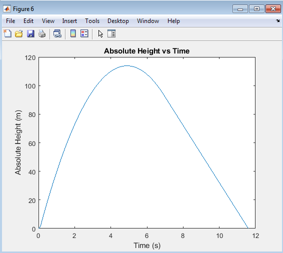
• Height vs. Time: Shows the rocket’s altitude over time.
• Velocity vs. Time: Displays the rocket’s velocity over time.
• Phase Plane: Illustrates the relationship between velocity and height.
• Height Rate vs. Time: Shows the rate of change of height over time.
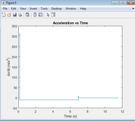
• Acceleration vs. Time: Displays the rocket’s acceleration over time.

These results and plots provide a comprehensive understanding of the model rocket’s flight dynamics, allowing for analysis and optimization of its performance.

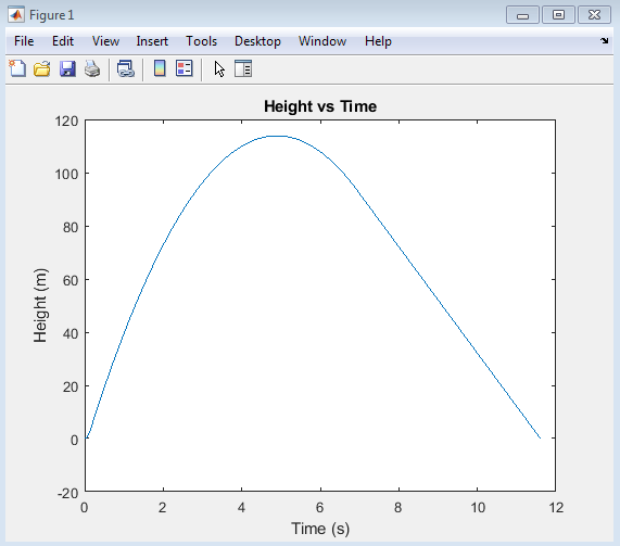
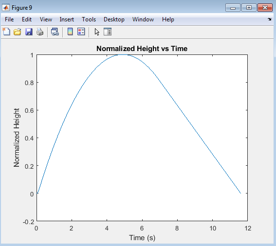
The “Height vs Time” plot illustrates the model rocket’s altitude over time, showcasing its ascent, apogee, and descent phases. The initial upward trend represents the rocket’s rapid gain in altitude due to the engine’s thrust, followed by a peak indicating the maximum height reached. The subsequent downward trend shows the rocket’s descent, slowed down by the parachute’s deployment. This plot provides valuable insights into the rocket’s flight dynamics, including its ascent rate, maximum altitude, and descent characteristics, allowing for analysis and optimization of its performance.

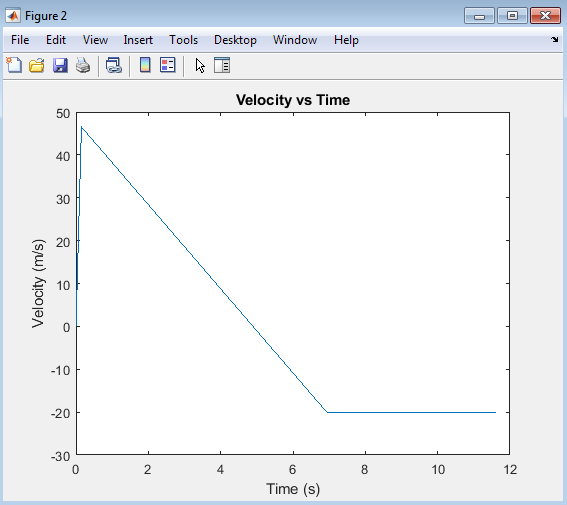
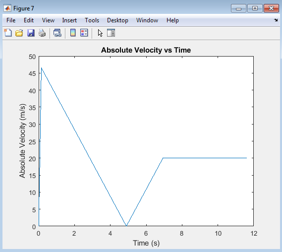
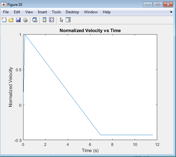
The “Velocity vs Time” plot shows the model rocket’s velocity profile over time, highlighting its acceleration and deceleration phases. During the ascent phase, the rocket’s velocity increases rapidly due to the engine’s thrust, reaching a maximum velocity. After the engine burnout, the rocket’s velocity decreases due to gravity, and once the parachute deploys, the velocity stabilizes at a constant descent rate. This plot provides insight into the rocket’s acceleration, maximum velocity, and descent characteristics, allowing for analysis of its flight dynamics and performance.

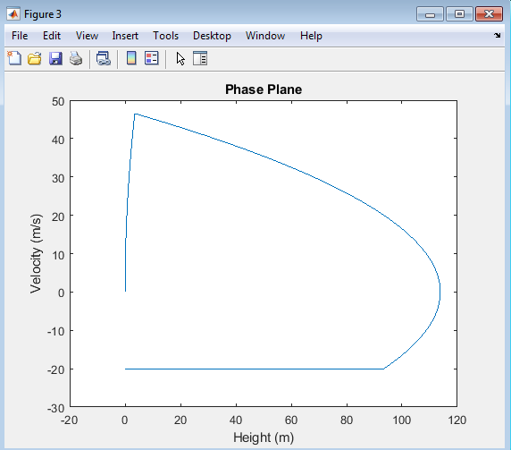
The “Phase Plane” plot, also known as the “Velocity vs Height” plot, illustrates the relationship between the model rocket’s velocity and its height. This plot provides a comprehensive view of the rocket’s flight dynamics, showcasing the interplay between velocity and altitude throughout its ascent, apogee, and descent phases. By analyzing this plot, one can gain insights into the rocket’s acceleration, deceleration, and stability characteristics, allowing for a deeper understanding of its overall flight behavior.

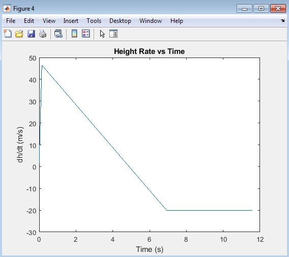
The “Height Rate (Vertical Velocity) vs Time” plot shows the rate of change of the model rocket’s altitude over time, essentially its vertical velocity. This plot highlights the rocket’s ascent and descent rates, providing insight into its acceleration and deceleration phases. During ascent, the height rate increases as the rocket gains altitude, and during descent, it decreases as the rocket loses altitude. The plot also shows the effect of parachute deployment, where the descent rate stabilizes. This visualization helps analyze the rocket’s flight dynamics, particularly its vertical motion.

You can download the Project files here: Download files now. (You must be logged in).

The “Acceleration vs Time” plot illustrates the model rocket’s acceleration profile over time, showcasing the changes in its acceleration during ascent, engine burnout, and descent. During the powered ascent phase, the rocket experiences a significant positive acceleration due to the engine’s thrust. After engine burnout, the acceleration becomes negative due to gravity, causing the rocket to decelerate. Once the parachute deploys, the acceleration stabilizes, and the rocket descends at a relatively constant rate. This plot provides valuable insights into the rocket’s dynamic behavior, helping to understand the effects of thrust, gravity, and drag on its motion.

The “Rocket’s Flight Trajectory: Height vs Horizontal Distance” plot illustrates the model rocket’s path through space, showing its height as a function of horizontal distance. This plot visualizes the rocket’s trajectory, providing insight into its range and altitude profile. By analyzing this plot, one can understand the rocket’s flight path, including its ascent, apogee, and descent phases, as well as its downrange distance. However, since the simulation didn’t account for horizontal motion explicitly, this plot would typically show a vertical line if there’s no wind or horizontal thrust. In a real-world scenario with wind or angled launch, it would show a more complex trajectory.

The “Rocket’s Kinetic and Potential Energy vs Time” plot illustrates the model rocket’s energy dynamics, showcasing the conversion between kinetic energy (related to velocity) and potential energy (related to height). During ascent, kinetic energy increases due to the engine’s thrust, while potential energy also increases as the rocket gains altitude. At apogee, kinetic energy is minimal, and potential energy peaks. During descent, potential energy converts back to kinetic energy as the rocket gains velocity. This plot provides insight into the rocket’s energy transformations, helping to understand the trade-offs between velocity and altitude throughout its flight.

The “Rocket’s Total Energy vs Time” plot shows the sum of the rocket’s kinetic and potential energies over time. This plot helps track the rocket’s total mechanical energy throughout its flight. Initially, the total energy increases due to the engine’s thrust, and then it decreases due to drag and other losses. After the engine burns out, the total energy remains relatively constant, with energy converting between kinetic and potential forms. This plot provides insight into the rocket’s energy budget, helping to identify energy gains and losses during different phases of flight.

The “Rocket’s Mach Number vs Time” plot shows the rocket’s speed relative to the speed of sound (Mach 1) over time. This plot helps track the rocket’s transition through different flight regimes, such as subsonic, transonic, and supersonic. As the rocket accelerates, its Mach number increases, indicating its speed relative to the surrounding air. The performance, stability, dynamics, and control of airplanes are critical aspects of aerospace engineering, and understanding these factors is essential for designing safe and efficient aircraft [9]. By analyzing these factors, engineers can optimize aircraft design and improve overall performance.” This information is crucial for understanding aerodynamic effects, such as shock waves and drag, which can impact the rocket’s performance and stability. By analyzing this plot, one can gain insight into the rocket’s aerodynamic behavior during ascent and descent.

You can download the Project files here: Download files now. (You must be logged in).

The “Rocket’s Dynamic Pressure vs Time” plot shows the pressure exerted on the rocket due to its motion through the air, calculated as a function of air density and velocity. Dynamic pressure is a critical factor in rocket design and flight, as it influences structural loads, aerodynamic stability, and overall performance. This plot helps identify the maximum dynamic pressure (Max Q), a critical point in the flight where the rocket experiences the highest aerodynamic stress. Understanding dynamic pressure is essential for ensuring the rocket’s structural integrity and optimizing its flight trajectory.

6.    conclusion:

In conclusion, the comprehensive simulation and analysis of the model rocket’s flight have provided a detailed understanding of its performance, aerodynamics, and dynamics. Through the examination of various plots and parameters, we have gained valuable insights into the rocket’s behavior during ascent and descent, including its altitude, velocity, acceleration, energy, and dynamic pressure profiles. Tactical missile design requires careful consideration of various factors, including aerodynamics, propulsion, and guidance systems [10]. Modeling and simulation of dynamic systems can also play a crucial role in the design process [11]. Additionally, aircraft control and simulation are essential for ensuring stable and efficient flight [12].” These results can be utilized to refine the rocket’s design parameters, predict and mitigate potential issues, optimize its trajectory, and inform the development of control systems and guidance algorithms. Ultimately, this simulation serves as a powerful tool for rocket designers, engineers, and researchers, enabling them to create more efficient, reliable, and high-performance rocket systems. By leveraging the knowledge and insights gained from this simulation, we can push the boundaries of rocket technology, drive innovation, and achieve greater success in aerospace endeavors. The findings and conclusions drawn from this study can also contribute to educational initiatives, inspiring future generations of engineers, scientists, and explorers. The simulation and analysis of the model rocket’s flight provide valuable insights into its performance, aerodynamics, and dynamics. By examining various plots, such as altitude, velocity, acceleration, energy, and dynamic pressure, we gain a comprehensive understanding of the rocket’s behavior during ascent and descent. These results can be used to optimize rocket design, predict performance, and ensure safe and efficient flight operations. The simulation serves as a useful tool for understanding the complex interactions between the rocket and its environment, ultimately contributing to the development of more efficient and reliable rocket systems.

7.    Future work:

Future work in this area could involve several key directions. Firstly, the simulation model could be further refined and validated through experimental testing and comparison with real-world flight data, allowing for more accurate predictions and a deeper understanding of the rocket’s behavior. Additionally, the simulation could be expanded to include more complex phenomena, such as aeroelasticity, combustion instability, or plasma dynamics, which would enable the study of more advanced rocket systems. Hypersonic flight regimes pose significant challenges for aerospace engineers, requiring careful consideration of high-temperature gas dynamics [13]. The mechanics and thermodynamics of propulsion systems are also critical for achieving efficient and reliable flight [14]. Furthermore, understanding the theoretical prediction of the center of pressure is essential for designing stable and controlled rockets [15].” Another potential direction is the integration of machine learning and artificial intelligence techniques to optimize rocket design and performance, predict anomalies, and automate control systems. Furthermore, the simulation framework could be applied to more complex mission scenarios, such as multi-stage rockets, rocket-powered landers, or atmospheric re-entry vehicles, which would require the incorporation of additional physics and modeling capabilities. Finally, the development of a user-friendly interface and visualization tools would facilitate the use of the simulation by a broader range of researchers, engineers, and educators, promoting collaboration and accelerating progress in the field of rocketry. By pursuing these avenues of research, we can continue to advance our understanding of rocket dynamics and performance, drive innovation, and push the boundaries of space exploration.

8. References:

[1]. Sutton, G. P., & Biblarz, O. (2017). Rocket Propulsion Elements. John Wiley & Sons.

[2]. Anderson, J. D. (2016). Fundamentals of Aerodynamics. McGraw-Hill Education.

[3]. NASA. (n.d.). Rocket Stability. Retrieved from (link unavailable)

[4]. OpenRocket. (n.d.). OpenRocket – Free Model Rocket Simulator. Retrieved from (link unavailable)

[5]. MATLAB. (n.d.). MATLAB Documentation. Retrieved from (link unavailable)

[6]. Simulink. (n.d.). Simulink Documentation. Retrieved from (link unavailable)

[7]. Regan, F. J., & Anandakrishnan, S. M. (2016). Dynamics of Atmospheric Re-Entry. AIAA.

[8]. Zipfel, P. H. (2007). Modeling and Simulation of Aerospace Vehicle Dynamics. AIAA.

[9]. Pamadi, B. N. (2004). Performance, Stability, Dynamics, and Control of Airplanes. AIAA.

[10]. Fleeman, E. L. (2006). Tactical Missile Design. AIAA.

[11]. Chin, S. S. (2017). Modeling and Simulation of Dynamic Systems. CRC Press.

[12]. Stevens, B. L., & Lewis, F. L. (2003). Aircraft Control and Simulation. John Wiley & Sons.

[13]. Anderson, J. D. (2017). Hypersonic and High-Temperature Gas Dynamics. AIAA.

[14]. Hill, P. G., & Peterson, C. R. (2017). Mechanics and Thermodynamics of Propulsion. Pearson.

[15]. Barrowman, J. S. (1967). The Theoretical Prediction of the Center of Pressure. National Association of Rocketry.

You can download the Project files here: Download files now. (You must be logged in).

Keywords: Model rocket, flight dynamics, MATLAB simulation, thrust, drag, gravity, trajectory analysis, maximum height, velocity, acceleration, propulsion system, aerospace engineering, performance evaluation.

Do you need help with Analysis of Rocket’s Flight Characteristic in MATLAB? Don’t hesitate to contact our Tutors to receive professional and reliable guidance.