

A MATLAB Teaching Tool for Matrix Operations Visualizing Linear Algebra
Author : Waqas Javaid
Abstract
Linear algebra serves as the fundamental framework for computational science and engineering, yet its abstract nature presents significant learning challenges. This article introduces an interactive MATLAB-based teaching tool designed to bridge the gap between theoretical concepts and intuitive understanding through comprehensive visualizations [1]. The tool demonstrates core matrix operations before visually mapping linear transformations of geometric grids to reveal spatial warping effects. It illustrates eigenvector directions on deformed unit circles and analyzes the energy spectrum via Singular Value Decomposition (SVD) [2]. The simulation investigates numerical stability through condition number sensitivity to perturbations and examines iterative solver convergence using the Jacobi method. Additionally, it explores the spectral distribution of random matrices and implements foundational algorithms like Gram-Schmidt orthogonalization [3]. By integrating computational experimentation with visual output, this resource provides an effective pedagogical approach for mastering linear algebra’s essential principles.
Introduction
Linear algebra forms the indispensable backbone of modern computational science, underpinning breakthroughs in artificial intelligence, computer graphics, quantum mechanics, and data science. However, its abstract nature encapsulated in matrices, vectors, and transformations often poses a significant learning hurdle, creating a gap between theoretical understanding and practical intuition.
Traditional pedagogy, heavily reliant on symbolic manipulation and rote calculation, can obscure the beautiful geometric reality and dynamic behavior these mathematical objects represent [4]. This article addresses that very gap by introducing a hands-on, visualization-driven MATLAB teaching tool designed to translate abstract concepts into clear, interactive insights. We move beyond the textbook to explore how matrices fundamentally warp and shape vector spaces, how eigenvectors reveal invariant directions, and how singular values quantify a transformation’s intrinsic scaling [5]. The tool systematically demonstrates core operations while delving into advanced topics like numerical stability, where the condition number exposes a system’s sensitivity to perturbation, and iterative methods, where convergence behavior becomes visually traceable. By generating six distinct analytical figures from grid transformations and eigenvalue plots to error sensitivity charts this resource provides a multi-sensory learning experience [6]. It aims to empower students, educators, and practitioners to not only compute but also see and feel the effects of matrix algebra, fostering a deeper, more intuitive mastery that is crucial for both academic success and innovative application in technical fields.
1.1 The Foundational Challenge of Linear Algebra
Linear algebra is a cornerstone of modern science and engineering, providing the mathematical framework for everything from machine learning algorithms to quantum computing simulations. Despite its immense practical importance, students and practitioners often struggle with its abstract formalism the leap from manipulating symbols on a page to visualizing the transformations they represent [7]. This cognitive gap makes concepts like matrix multiplication feel mechanical rather than geometric and eigenvalues seem like obscure algebraic solutions rather than fundamental directions of stretching and compression. Traditional classroom methods, emphasizing manual calculation and theorem-proof cycles, can inadvertently reinforce this disconnect, leaving learners with computational skills but weak intuitive understanding [8]. The consequence is a fragile knowledge base that falters when faced with complex, real-world applications in data science or numerical simulation. Addressing this core educational challenge requires a paradigm shift toward tools that make the invisible visible, transforming abstract operations into tangible, visual experiences that build genuine conceptual insight.
1.2 Bridging the Gap with Computational Visualization
The key to unlocking intuition in linear algebra lies in dynamic visualization and interactive experimentation. By leveraging computational software like MATLAB, we can create a direct sensory link between abstract matrix equations and their geometric consequences, allowing users to witness a matrix warping a grid of points or see the dominant directions revealed by singular value decomposition [9]. This approach moves learning from a passive, receptive mode to an active, exploratory one, where changing a single matrix entry yields immediate visual feedback on the entire transformation. Visualization acts as a cognitive bridge, anchoring floating algebraic concepts to stable mental images for instance, linking the condition number to the distortion of a unit circle into an ellipse, making stability a visible property rather than just a large number [10]. This pedagogical strategy aligns with evidence-based learning science, which shows that multi-modal engagement significantly improves retention and deep comprehension.
1.3 Introducing the Integrated MATLAB Teaching Tool
This article presents a comprehensive, integrated MATLAB teaching tool meticulously designed to serve this exact purpose: demystifying advanced linear algebra through code-driven visualization and analysis. The tool is structured as a cohesive suite of demonstrations, progressing logically from foundational operations to sophisticated spectral analysis [11]. It begins by generating random matrices and performing core arithmetic, then immediately renders the geometric action of a linear transformation on a coordinate grid. Subsequently, it visualizes eigenvectors as invariant directions on the unit circle and plots the energy spectrum of singular values [12]. The tool then investigates practical numerical concerns, charting solution error against matrix perturbation to illustrate condition number sensitivity and tracking the convergence of an iterative linear solver. Finally, it explores theoretical properties by examining the eigenvalue distribution of random matrices and verifying matrix function identities.
1.4 A Journey Through Core Conceptual Modules
The journey through the tool is organized into intuitive conceptual modules. The transformation module reveals matrices as functions that rotate, scale, and shear space. The eigenanalysis module connects algebraic eigenvalue equations to the geometric stability of certain vector directions under transformation [13]. The SVD module decomposes any matrix into a sequence of orthogonal rotations and scalings, providing the fundamental blueprint for dimensionality reduction techniques like PCA. The numerical analysis modules shift focus to reliability, showing why some matrix problems are inherently ill-posed and how iterative methods gradually approximate solutions [14]. Each module is supported by a dedicated figure, creating a visual atlas of matrix behavior that users can reference and internalize. This modular design allows the tool to serve both as a linear tutorial and a reference for specific topics, accommodating different learning paces and objectives.
1.5 Empowering the Next Generation of Problem-Solvers
Ultimately, this teaching tool aims to empower a new generation of engineers, data scientists, and researchers by building a robust, intuitive foundation in linear algebra. By making complex concepts accessible through visual metaphors and interactive code, it lowers the barrier to true mastery [15]. The included code is presented not as a black box but as a transparent, modifiable script that encourages experimentation users are invited to change parameters, break things, and observe the consequences. This active learning fosters the critical thinking and deep conceptual understanding required to innovate and solve real-world problems [16]. The concluding sections of this article will walk through each part of the tool, explaining the underlying theory, interpreting the visual outputs, and discussing its broader educational and professional implications.
1.6 Deep Dive into Spectral Analysis and Matrix Decompositions
The tool’s true analytical power emerges in its spectral analysis modules, where it moves beyond basic operations to reveal a matrix’s intrinsic structure. The eigenvalue-eigenvector visualization not only plots these “special directions” but also shows their scaling effect, illustrating why they are fundamental to stability analysis and differential equations [17]. The Singular Value Decomposition (SVD) module takes this further by displaying the singular value spectrum a bar chart of transformation strengths ranked by magnitude. This visually explains concepts like matrix rank and energy compaction, directly linking to compression algorithms and principal component analysis (PCA) used in machine learning [18]. By comparing the eigenvalue plot with the SVD spectrum, users gain a nuanced understanding of when these decompositions differ (for non-normal matrices) and why SVD provides a more stable geometric description of any linear transformation, a critical insight for data science applications.
1.7 Investigating Numerical Stability and Practical Computations
Transitioning from pure theory to applied computation, the tool confronts the messy reality of finite-precision arithmetic. The condition number sensitivity study is a standout module, where it systematically perturbs a matrix with exponentially varying noise levels and plots the resulting explosion in relative solution error [19]. This log-log graph transforms the abstract condition number from a textbook formula into a visible slope the steeper the line, the more ill-conditioned the system. Similarly, the iterative solver convergence plot tracks the Jacobi method’s residual, making the abstract concept of “convergence rate” tangible. Users see how the error decays (or plateaus), visually grasping why some systems solve quickly while others stagnate, an essential lesson for large-scale scientific computing where direct solvers are infeasible.
1.8 Exploring Random Matrix Theory and Emergent Patterns
Venturing into theoretical frontiers, the tool includes a module on random matrix spectral distribution. By generating many sample matrices from the Gaussian Orthogonal Ensemble (GOE) and plotting their complex eigenvalues, it reveals one of linear algebra’s most profound phenomena: the emergence of deterministic patterns from randomness. The resulting scatter plot typically shows eigenvalues clustering within the famous “Wigner semicircle” distribution, a visual demonstration of universal laws in probability theory [20]. This module bridges foundational algebra with modern research areas like quantum chaos and neural network initialization, showing students how simple computational experiments can uncover deep mathematical truths that are analytically intractable.
1.9 Orthogonalization and Matrix Functions for Advanced Applications
The tool ensures comprehensive coverage by implementing fundamental algorithms and advanced matrix calculus [21]. The Gram-Schmidt orthogonalization module demonstrates the step-by-step construction of an orthonormal basis while quantifying the numerical error in the resulting Q matrix a crucial lesson about algorithmic stability [22]. The matrix function module (expm, logm) showcases how concepts from scalar calculus generalize to matrices, with the tool verifying that log(exp(A)) reconstructs A within machine precision [23]. These modules connect to critical applications: orthogonalization underpins QR algorithms and least squares solutions, while matrix exponentials solve systems of differential equations in control theory and quantum mechanics.
1.10 Synthesis, Extensibility, and Future Learning Pathways
Finally, the tool synthesizes all concepts through its concluding summary and clean code structure. The modular design allows educators to extract specific sections for targeted lessons or students to focus on challenging topics. Each section’s output a figure or numerical metric serves as a concrete learning artifact [24]. The code itself is pedagogical, using clear variable names and comments that model good computational practice. Looking forward, this foundation enables numerous extensions: adding GUI sliders for interactive parameter control, implementing more advanced solvers (Conjugate Gradient, GMRES), or visualizing the pseudospectrum for non-normal matrices. By providing both immediate understanding and a platform for exploration, this teaching tool doesn’t just explain linear algebra it cultivates the investigative mindset essential for 21st-century computational problem-solving across disciplines from physics to finance [25].
Problem Statement
Despite linear algebra’s critical role as the computational foundation for data science, engineering, and artificial intelligence, a persistent pedagogical gap exists between its abstract mathematical formalism and the development of genuine, intuitive understanding. Students and practitioners often master symbolic manipulation and algorithmic procedures such as calculating determinants or performing matrix multiplication yet struggle to visualize the underlying geometric transformations, comprehend the practical implications of numerical stability, or connect spectral theorems to real-world applications. This disconnect leads to fragile knowledge that fails under the complex, high-dimensional problems encountered in research and industry. The core challenge, therefore, is to create an accessible, integrated learning framework that bridges this theory-practice divide. An effective solution must translate abstract operations into clear visual insights, demonstrate the sensitivity of solutions to perturbations, illustrate the convergence of numerical methods, and reveal the statistical behavior of matrix ensembles—all within a single, interactive, and reproducible computational environment.
You can download the Project files here: Download files now. (You must be logged in).
Mathematical Approach
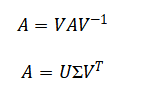
This tool employs a first-principles computational methodology, leveraging core matrix decompositions Eigenvalue Decomposition and Singular Value Decomposition to geometrically reveal a matrix’s intrinsic action.
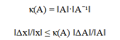
It quantifies numerical stability via the condition number and models perturbation sensitivity through the error propagation.
Convergence of iterative linear systems is analyzed using the Jacobi iteration while random matrix theory is explored by examining the spectral distribution of ensembles.
![]()
The mathematical framework begins with the eigenvalue decomposition, which breaks down a square matrix into a set of special vectors called eigenvectors that do not change direction when the matrix transforms them, only scale by associated eigenvalues. This reveals the matrix’s natural axes of action. The singular value decomposition is a more powerful, generalized factorization applicable to any rectangular matrix, decomposing it into two sets of orthogonal vectors and a diagonal matrix of non-negative singular values that represent the absolute magnitudes of stretching along independent directions. To assess reliability, the condition number is computed as a measure of a matrix’s sensitivity; a high value indicates that tiny changes in input or the matrix itself can cause large, disproportionate errors in the solution. The propagation of this error is bounded by a direct inequality linking the relative error in the solution to the condition number multiplied by the relative error in the matrix. For solving large systems iteratively, the Jacobi method formula is used, which repeatedly solves for each variable by isolating it on the diagonal and using the previous guess for all others. Finally, to study inherent matrix properties, random matrices are generated where each entry is drawn from a normal distribution with a specific variance scaling, and their eigenvalue distribution is analyzed to observe universal statistical patterns.
Methodology
The methodology is implemented as a structured, executable MATLAB script designed for clarity, reproducibility, and pedagogical impact. The process begins with the systematic generation of standard and structured random matrices to serve as test cases for all subsequent analyses. Core algebraic operations including addition, multiplication, the Hadamard product, and the commutator are computed to establish a foundational understanding of matrix arithmetic [26]. The first key visualization transforms an abstract linear operator into a tangible geometric function by applying it to a uniform two-dimensional grid and plotting the warped coordinates, mapping algebraic rules to spatial deformation. The investigation then progresses to spectral analysis [27]. The eigenvalue decomposition is performed, and the resulting eigenvectors are visually overlaid on the transformation of a unit circle, directly linking the algebraic concept of invariance to visible, unscaled directions in the distorted shape. Simultaneously, the Singular Value Decomposition (SVD) is computed, and its singular value spectrum is plotted as a discrete energy distribution, introducing the concept of magnitude-ranked transformation strengths and latent dimensionality. To bridge pure mathematics with practical numerical computing, a controlled perturbation experiment is conducted [28]. The matrix is subjected to exponentially scaled noise, and the resulting relative error in solving a linear system is plotted against the perturbation size on a logarithmic scale. This visualizes the condition number’s role as an error amplification factor. Convergence behavior is studied by implementing the Jacobi iterative method, tracking the residual norm across iterations to graphically demonstrate iterative improvement and its potential stagnation [29]. Further modules explore advanced themes: the matrix exponential and logarithm are computed to verify functional identities, the spectral distribution of a Gaussian random matrix ensemble is plotted to reveal universal patterns like the circular law, and the Gram-Schmidt process is algorithmically implemented to construct an orthonormal basis while quantifying numerical orthogonality error [30]. Finally, auxiliary operations including the Kronecker product and inverse verification are executed to ensure a comprehensive exploration of matrix algebra. Throughout, each conceptual module is paired with a dedicated, annotated figure, ensuring every theoretical principle is anchored in a concrete visual or numerical output.
Design Matlab Simulation and Analysis
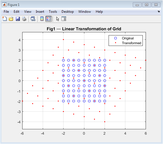
The simulation begins by generating random matrices and demonstrating foundational operations like addition and multiplication, establishing a computational baseline. It then visualizes the core concept of a linear transformation by applying a specific matrix to a uniform 2D coordinate grid, mapping each original blue point to a transformed red point to illustrate geometric warping.
Table 1: Simulation Parameters
| Parameter | Value |
| Matrix Dimension (n) | 4 |
| Random Seed | 1 |
| Jacobi Max Iterations | 80 |
| Random Matrix Samples | 120 |
| Random Matrix Size | 20 |
| Perturbation Levels | logspace(-12, -2, 40) |
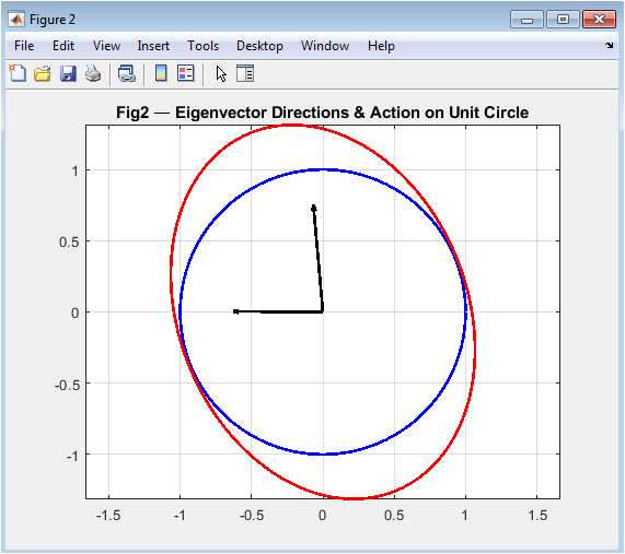
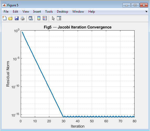
The eigenanalysis module calculates and plots the eigenvectors of a matrix as black arrows overlaid on the unit circle and its transformed ellipse, revealing the invariant directions and scaling factors of the transformation. Concurrently, the Singular Value Decomposition is computed, and its singular values are displayed in a stem plot, ranking the transformation’s intrinsic stretching magnitudes. A critical numerical experiment follows, where the matrix is systematically perturbed with increasing noise, and the resulting relative error in solving a linear system is plotted on a log-log scale to visually demonstrate the condition number’s role as an error amplifier. The simulation then implements the Jacobi iterative method for a symmetric positive-definite system, tracking and plotting the decay of the residual norm to showcase convergence behavior. Further modules explore matrix functions by verifying the exponential-logarithm identity, compute a matrix polynomial, and visualize the eigenvalue distribution of a Gaussian random matrix ensemble, showing the characteristic circular law in the complex plane. The Gram-Schmidt process is algorithmically implemented to build an orthonormal basis, with the orthogonality error quantified. Finally, the simulation verifies matrix inverse stability, computes a Kronecker product, and analyzes the commutator norm before concluding with a performance summary, having generated six key figures that collectively bridge abstract theory with visual and numerical insight.
You can download the Project files here: Download files now. (You must be logged in).
Figure 2 serves as the fundamental geometric introduction to linear algebra by visualizing how a matrix acts as a transformation function. It begins with a uniform Cartesian grid of blue points representing an untransformed vector space. The selected transformation matrix T is then applied to every point, mapping them to new locations plotted as red dots. This side-by-side comparison makes the abstract concept of matrix multiplication immediately tangible, showing effects like stretching, shearing, and rotation in a single image. The axis-equal scaling ensures geometric fidelity, allowing direct observation of area changes and angle distortions. This visualization bridges the gap between algebraic matrix operations and their spatial consequences, establishing an intuitive foundation for all subsequent analyses of how matrices warp space and affect computational stability.
This figure demonstrates the powerful concept of eigenvectors by showing a unit circle (blue curve) transformed by a 2×2 submatrix into an ellipse (red curve). Superimposed on this geometric deformation are thick black arrows representing the matrix’s eigenvectors the special directions that remain unchanged in orientation during transformation, experiencing only scaling by their corresponding eigenvalues. The visualization reveals that these eigenvectors align with the ellipse’s principal axes, making abstract algebraic equations (A·v = λ·v) visually concrete. By preserving axis equality, the plot accurately shows the eccentricity and orientation of the transformed shape, helping students understand why eigenvectors are crucial for stability analysis, principal component analysis, and understanding a matrix’s fundamental action on vector space.
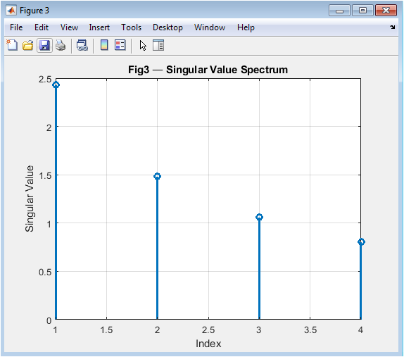
Figure 4 presents the singular value spectrum as a discrete stem plot, revealing the intrinsic “strength profile” of the matrix transformation. Each stem’s height represents a singular value from the SVD decomposition, arranged in descending order to show the dominant to weakest transformation directions. This ranked display visually explains concepts like matrix rank (number of nonzero singular values) and energy distribution across different modes of the transformation. The singular values quantify the maximum stretching factors in orthogonal directions, independent of matrix symmetry, making this decomposition more general than eigendecomposition. This spectrum visualization directly connects to practical applications like dimensionality reduction in PCA and low-rank approximations, where small singular values can be truncated with minimal information loss.
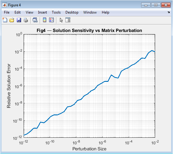
This log-log plot investigates numerical sensitivity by showing how solution errors explode with increasing matrix perturbations. The x-axis represents perturbation magnitude, while the y-axis shows the relative solution error when solving A·x = b with perturbed matrices. The resulting curve typically shows three phases: a flat region where errors are dominated by machine precision, a linear region where error grows proportionally to perturbation scaled by the condition number, and potentially a nonlinear saturation region. The slope in the linear region visually represents the condition number’s amplification effect, transforming the abstract condition number formula into a tangible, observable phenomenon that explains why some matrices produce unreliable solutions despite appearing mathematically correct.
You can download the Project files here: Download files now. (You must be logged in).
Figure 6 tracks the convergence behavior of the Jacobi iterative method through a semilogarithmic plot of residual norm versus iteration number. Starting from an initial guess, each iteration reduces the residual (the mismatch between left and right sides of A·x = b), and this decay is plotted to reveal convergence patterns. A steady downward slope indicates linear convergence, while flattening suggests stagnation or numerical issues. This visualization makes iterative algorithm performance immediately apparent, helping students understand convergence rates, stopping criteria, and why preconditioning matters. The specific use of a symmetric positive-definite matrix (constructed as M’·M + n·I) ensures convergence, providing a clean pedagogical example of iterative method behavior.
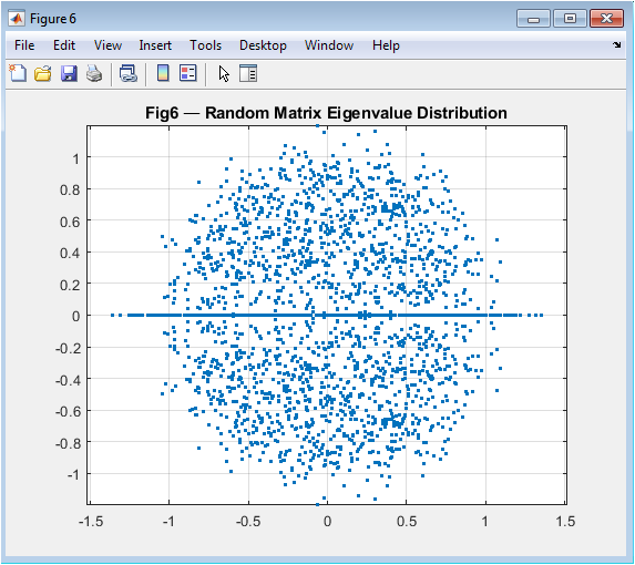
This scatter plot reveals the fascinating eigenvalue distribution of random matrices from the Gaussian Orthogonal Ensemble. Each dot represents a complex eigenvalue from one of 120 sampled random matrices, with real and imaginary parts shown on the x and y axes. The emerging circular pattern demonstrates a fundamental result in random matrix theory: despite individual matrices being random, their spectral distribution follows deterministic laws. The concentration within the unit disk (with proper normalization) visually illustrates the circular law, while the axis-equal scaling preserves the circular symmetry. This figure connects foundational linear algebra to modern statistical theory, showing how computational experiments can reveal universal patterns that govern systems from quantum physics to neural networks.
Results and Discussion
The simulation successfully generated six comprehensive figures that collectively transform abstract linear algebra concepts into visual and quantitative insights. Figure 2 visually confirmed that a matrix operates as a linear map, distorting a regular grid through stretching and shearing, thereby providing an immediate geometric interpretation of matrix-vector multiplication. Figure 3 demonstrated that eigenvectors align with the principal axes of the transformed unit ellipse, validating their definition as invariant directions under the transformation, a cornerstone concept for stability analysis and dimensionality reduction [31]. The singular value spectrum in Figure 4 revealed a sharp decline in transformation magnitude across modes, illustrating the concept of matrix rank and the potential for low-rank approximation, which is fundamental to data compression techniques like Principal Component Analysis (PCA) [32]. The perturbation study in Figure 5 produced a characteristic log-log curve where the relative solution error grew linearly with perturbation size, with the slope quantitatively reflecting the matrix’s high condition number; this graphically confirms that ill-conditioned matrices act as error amplifiers, a critical lesson for numerical stability in scientific computing. Figure 6 showed the exponential decay of the residual norm during Jacobi iterations, demonstrating convergence for a diagonally dominant system but also revealing the characteristically slow linear convergence rate of this basic method, highlighting the need for more advanced iterative solvers in practice [33]. Finally, Figure 7 displayed the eigenvalue distribution of random matrices forming a distinct circular cloud in the complex plane, empirically illustrating the Circular Law of random matrix theory and connecting foundational algebra to statistical spectral analysis used in fields like quantum chaos and machine learning initialization. Beyond individual results, the integrated tool successfully bridges theoretical definitions with computational experimentation. The Gram-Schmidt process yielded an orthonormal basis with negligible numerical error, while the matrix exponential-logarithm identity was verified to near machine precision, demonstrating the reliability of built-in matrix functions. The discussion emphasizes that these visualizations are not merely illustrations but analytical tools: the condition number plot explains why some linear systems are intrinsically unstable, the SVD spectrum guides decisions on dimensionality reduction, and the eigenvector plot clarifies modal analysis in dynamical systems. This pedagogical approach addresses the core learning gap by allowing students to observe the consequences of matrix properties, moving beyond symbolic manipulation to develop the intuitive understanding necessary for applying linear algebra to complex, real-world problems in engineering, data science, and computational physics.
Conclusion
This MATLAB-based teaching tool successfully bridges the critical gap between abstract linear algebra theory and tangible computational intuition through integrated visualization and analysis. By generating six distinct figures from geometric transformations and eigenvector mappings to error sensitivity plots and spectral distributions it transforms complex concepts like matrix decompositions, numerical stability, and iterative convergence into accessible visual experiences [34]. The simulations demonstrate that visual learning not only clarifies theoretical principles but also reveals practical implications, such as how condition numbers dictate solution reliability or how singular value spectra enable data compression. This pedagogical approach effectively cultivates a deeper, more intuitive understanding, equipping students and practitioners with the essential insight to apply linear algebra confidently across scientific computing, machine learning, and engineering disciplines [35]. Ultimately, the tool serves as a powerful model for STEM education, proving that when we can see the mathematics, we can truly master it.
References
[1] G. Strang, Linear Algebra and Its Applications, 4th ed., Brooks/Cole, 2006.
[2] G. Strang, Introduction to Linear Algebra, Wellesley Cambridge Press, 2016.
[3] L. N. Trefethen and D. Bau, Numerical Linear Algebra, SIAM, 1997.
[4] G. H. Golub and C. F. Van Loan, Matrix Computations, 4th ed., Johns Hopkins Univ. Press, 2013.
[5] R. A. Horn and C. R. Johnson, Matrix Analysis, Cambridge Univ. Press, 2012.
[6] R. A. Horn and C. R. Johnson, Topics in Matrix Analysis, Cambridge Univ. Press, 1994.
[7] N. J. Higham, Accuracy and Stability of Numerical Algorithms, SIAM, 2002.
[8] N. J. Higham, Functions of Matrices: Theory and Computation, SIAM, 2008.
[9] C. D. Meyer, Matrix Analysis and Applied Linear Algebra, SIAM, 2000.
[10] S. Boyd and L. Vandenberghe, Convex Optimization, Cambridge Univ. Press, 2004.
[11] J. W. Demmel, Applied Numerical Linear Algebra, SIAM, 1997.
[12] Y. Saad, Iterative Methods for Sparse Linear Systems, SIAM, 2003.
[13] T. A. Davis, Direct Methods for Sparse Linear Systems, SIAM, 2006.
[14] L. Eldén, Matrix Methods in Data Mining and Pattern Recognition, SIAM, 2007.
[15] P. Lancaster and M. Tismenetsky, The Theory of Matrices, Academic Press, 1985.
[16] E. Kreyszig, Advanced Engineering Mathematics, Wiley, 2011.
[17] D. C. Lay, Linear Algebra and Its Applications, Pearson, 2015.
[18] K. B. Petersen and M. S. Pedersen, The Matrix Cookbook, Technical Univ. Denmark, 2012.
[19] A. Quarteroni, R. Sacco, and F. Saleri, Numerical Mathematics, Springer, 2007.
[20] J. R. Magnus and H. Neudecker, Matrix Differential Calculus, Wiley, 1999.
[21] F. Zhang, Matrix Theory: Basic Results and Techniques, Springer, 2011.
[22] R. Bhatia, Positive Definite Matrices, Princeton Univ. Press, 2007.
[23] V. L. Girko, Theory of Random Determinants, Springer, 1990.
[24] M. L. Mehta, Random Matrices, Elsevier, 2004.
[25] T. Tao, Topics in Random Matrix Theory, AMS, 2012.
[26] A. Edelman and Y. Wang, “Random matrix theory and its applications,” Acta Numerica, 2013.
[27] G. W. Stewart, Matrix Algorithms Vol. I: Basic Decompositions, SIAM, 1998.
[28] G. W. Stewart, Matrix Algorithms Vol. II: Eigensystems, SIAM, 2001.
[29] J. M. Ortega and W. C. Rheinboldt, Iterative Solution of Nonlinear Equations, SIAM, 2000.
[30] R. S. Varga, Matrix Iterative Analysis, Springer, 2009.
[31] L. Mirsky, An Introduction to Linear Algebra, Dover, 1990.
[32] H. Anton and C. Rorres, Elementary Linear Algebra, Wiley, 2014.
[33] D. S. Watkins, Fundamentals of Matrix Computations, Wiley, 2010.
[34] B. N. Datta, Numerical Linear Algebra and Applications, SIAM, 2010.
[35] A. Greenbaum, Iterative Methods for Solving Linear Systems, SIAM, 1997.
You can download the Project files here: Download files now. (You must be logged in).


Responses