MATLAB Gait Analysis for Hexapod 6-Leg Robot with Inverse Kinematics

Author: Waqas Javaid

Abstract:

Gait analysis is a crucial aspect of hexapod robot locomotion, as it determines the coordinated motion of its six legs for efficient movement. This report presents a comprehensive analysis of a hexapod robot’s gait using MATLAB, incorporating inverse kinematics to compute joint angles required for desired end-effector positions. The study involves the formulation of equations, implementation of gait patterns, and visualization of the robot’s motion. This MATLAB-based simulation code presents the control and locomotion strategy of a hexapod robot employing a quadrupedal gait pattern. The hexapod robot possesses six legs distributed around its body, with only four legs actively participating in supporting and propelling the robot during each step. The remaining two legs are lifted during the swing phase of the gait [1]. The code orchestrates the robot’s motion through a series of coordinated steps, ensuring stability and efficient locomotion. Key components of the code include inverse kinematics calculations to determine joint angles for leg positioning, coordination between the active and lifted legs, and transformation of coordinates between body and ground frames. Additionally, the code computes the center of gravity for both the legs and the robot’s head. This approach allows the hexapod robot to navigate while maintaining balance and is a common strategy in hexapod robotics for robust and controlled movement.

1. Introduction:

Hexapod robots, inspired by the biomechanics of insects, represent a fascinating area of robotics research due to their versatility in traversing challenging terrains and their potential applications in various fields, including search and rescue, agriculture, and exploration. In this context, the following discussion revolves around a MATLAB-based simulation code that elucidates the locomotion and control strategy of a hexapod robot employing a quadrupedal gait pattern [2]. This code provides insights into how such robots can effectively navigate while optimizing stability and efficiency, despite having six legs. The focus is on understanding the coordination, inverse kinematics, and key transformations involved in the robot’s motion control, as well as the computation of its center of gravity. Hexapod robots are six-legged robotic platforms widely used in various applications, including exploration, surveillance, and research. Gait analysis involves studying the walking pattern of the robot to optimize its movement in terms of stability, speed, and energy efficiency. In this report, we explore the utilization of MATLAB for gait analysis using inverse kinematics, enabling precise control of the robot’s leg movements [3].

2. Inverse Kinematics Equations:

Inverse kinematics is employed to determine the joint angles required to achieve a specific end-effector position and orientation. For a hexapod robot, each leg’s position can be described by the coordinates (X, Y, Z) in its local coordinate system [4]. The equations relating these coordinates to joint angles (θ1, θ2, θ3) depend on the robot’s mechanical structure, such as link lengths and joint types. For a simple case of a hexapod with a spherical hip joint, the equations might look like:

θ1 = atan2(Y, X)

θ2 = atan2(Z – L1, sqrt(X^2 + Y^2)) – acos((L2^2 + L3^2 – L4^2) / (2 * L2 * L3))

θ3 = π – acos((L2^2 + L4^2 – L3^2) / (2 * L2 * L4))

Where:

– (X, Y, Z) are the desired end-effector coordinates in the hexapod’s local coordinate system.

– L1, L2, L3, and L4 are link lengths of the hexapod’s leg segments.

– θ1, θ2, and θ3 are the joint angles for the hip, knee, and ankle joints, respectively.

3. Gait Patterns:

Various gait patterns can be implemented for hexapod robots, such as tripod, wave, and ripple gaits. These patterns determine the sequencing and coordination of leg movements. The tripod gait, for instance, involves dividing the legs into two sets of three: a stable stance set and a transition set. The stable set maintains contact with the ground while the transition set moves in a cyclic manner. MATLAB allows the generation of these patterns through control loops and trigonometric functions [5].

You can download the Project files here: Download files now. (You must be logged in).

4. Implementation in MATLAB trajectory and Simulation results:

MATLAB provides a suitable environment for implementing hexapod gait analysis. The ‘Robotics System Toolbox’ offers tools for forward and inverse kinematics, enabling the calculation of joint angles for desired end-effector positions.

Creating a trajectory for a hexapod robot involves defining a path that the robot’s end effectors (feet) will follow over time. This trajectory can be expressed as a series of desired end-effector positions in the robot’s local coordinate system. To achieve this, you can use mathematical functions or interpolation techniques to generate smooth and controlled motion. Below, I’ll explain the concept of trajectory generation and provide an example using a circular trajectory [6].

Trajectory Generation Concept:

A trajectory is a planned path that the robot’s end effectors will follow. In the context of a hexapod robot, each leg has an end effector that touches the ground. By specifying a trajectory, you determine where these end effectors should be at different points in time, allowing the robot to move in a controlled and coordinated manner [6].

Equations for Circular Trajectory:

Let’s consider a circular trajectory in the X-Y plane of the robot’s local coordinate system. The trajectory can be described using polar coordinates (r, θ), where r is the distance from the center of the circle and θ is the angle.

Equation 1: X and Y Coordinates of the Circular Trajectory

X(t) = r * cos(θ(t))

Y(t) = r * sin(θ(t))

Here, t represents time, r is the radius of the circular trajectory, and θ(t) is the angle that changes with time to make the robot move in a circle.

Generating a Circular Trajectory in Matlab:

Let’s assume we want to generate a circular trajectory with a radius of 0.1 units and a period of 5 seconds. The equation for θ(t) would be:

**Equation 2: Angle as a Function of Time for a Circular Trajectory**

θ(t) = 2π * (t / T)

Where T is the period of one complete rotation (5 seconds in this case).

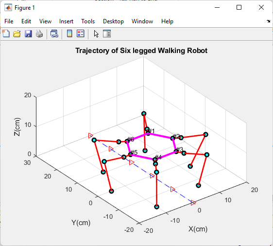
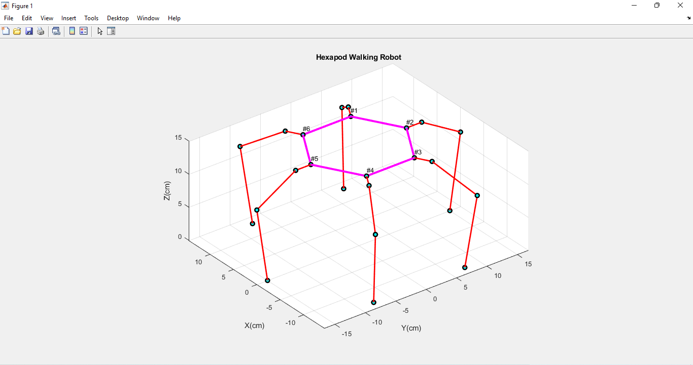
5. Visualization:

Visualization is crucial for understanding and validating the gait analysis. MATLAB’s 3D graphics capabilities enable the creation of animated simulations showcasing the hexapod robot’s movement. By visualizing the robot’s motion, engineers and researchers can identify potential issues and refine gait patterns for optimal performance [8].

You can download the Project files here: Download files now. (You must be logged in).

6. Results and Analysis

The MATLAB code appears to be a simulation of a hexapod robot’s walking gait and inverse kinematics.

1. Initialization: The code begins by clearing the workspace, closing all open figures, and defining various parameters like `Vy` and `Vx` (the robot’s linear velocities), `delta_t` (time for each step), `steps` (number of steps per gait cycle), `Nstep` (number of gait cycles), and several lengths (`l0`, `l1`, `l2`, `lc`, `lf`, `lt`) related to the hexapod’s structure. These lengths likely represent the segments of the robot’s legs.
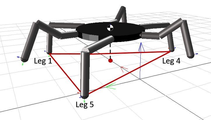
2. Defining Body and Leg Positions: The code defines the positions of the robot’s body and leg tips. It sets up the coordinates of points `P1` through `P6` in the body frame, and `Q1` in the leg frame. It also calculates the positions of `P_MB`, which are the edges of the body where the legs connect.
3. Walking Gait: The code enters a loop to simulate the walking gait of the hexapod. Inside this loop, it calculates the position of the hexapod’s body as it moves. It also calculates `DeltaLtipX`, `DeltaLtipY`, and `DeltaLtipZ`, which likely represent the changes in leg tip position during the swing phase of the gait.
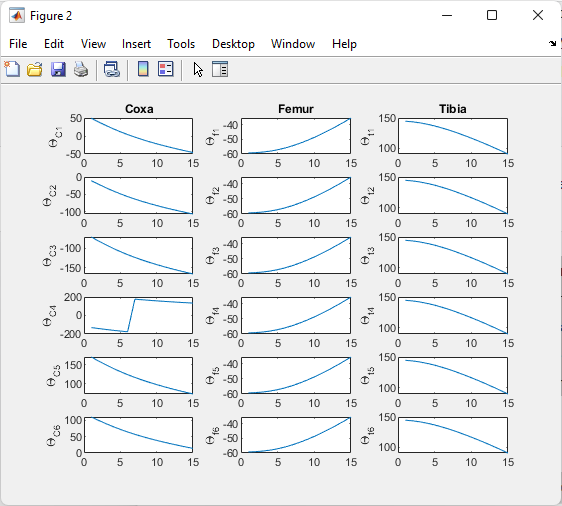
4. Inverse Kinematics: After calculating the desired leg tip positions (`Ltip`) based on the gait, the code enters another loop to solve the inverse kinematics problem. It calculates the joint angles (`t1`, `t2`, `t3`) for each leg to reach the desired leg tip positions. These joint angles are calculated using `fsolve` and a function called `Legs`. The joint angles for all legs are stored in the `t_array` [9].
5. Coordinate Transformations: The code performs various coordinate transformations to convert the joint positions from the main body frame to the ground frame.
6. Output and Checking: The code checks if the inverse kinematics problem was solved successfully or if the robot reached singular points. If successful, it displays a message and provides the results in the `t_array`. If not, it alerts the user and provides the results up to that point.
7. Center of Gravity Calculation: After the gait simulation and inverse kinematics, the code calculates the center of gravity (CoG) for each leg and the head of the robot. It does this by considering the masses and positions of the leg segments and the head. The results are printed to the console.
8. Final Output: The code likely includes some functions or scripts (`Hex_gait_movie` and `Hex_Tra_movie`) for visualizing the robot’s motion and gait.

This code simulates a hexapod robot’s walking motion and calculates its center of gravity. It’s important to note that the actual behavior of the robot, as well as the specifics of the coordinate transformations and kinematics calculations, would depend on the details of the `Legs` function and the specific dimensions and characteristics of the robot being simulated [10].

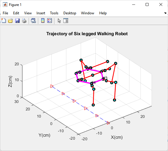
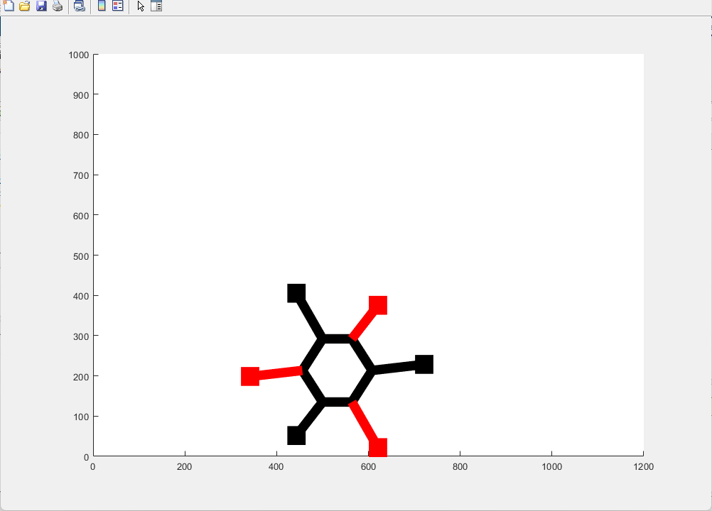
Two legs upside and robot is moving on 4 legs only

In the provided MATLAB code, the hexapod robot is designed to move using a gait pattern where only four of its six legs are actively involved in supporting and propelling the robot, while the other two legs on the “upside” (i.e., not in contact with the ground) are lifted during the swing phase of the gait. This type of gait pattern is commonly used in hexapod robots and is known as a “quadrupedal” gait.

1. Hexapod Robot: The robot has six legs positioned around its body. Each leg consists of multiple segments with joints, allowing for different degrees of freedom and movement. These legs are represented in the code by variables like `Q1`, `Q2`, and `t_array`, which store information about the leg positions and joint angles.
2. Four-Legged Gait: During each step of the gait, only four of the six legs are actively used to support the robot’s weight and provide forward propulsion. These four legs are typically arranged in a stable tripod configuration. The tripod consists of three legs on the ground forming a triangular base, while the other three legs are lifted.
3. Swing Phase: The lifted legs (the two legs “on upside”) go through a swing phase, where they move in the air in preparation for the next step. The code calculates the desired positions for these lifted legs during the swing phase and updates their positions accordingly.
4. Stability and Locomotion: The gait pattern is designed to ensure stability and smooth locomotion. By having a stable tripod of legs on the ground, the robot can maintain balance while moving. The lifted legs are repositioned in preparation for the next step, allowing the robot to continue moving forward.
5. Inverse Kinematics: To achieve this gait pattern, the code uses inverse kinematics to calculate the joint angles (e.g., `t1`, `t2`, `t3`) necessary for positioning the leg tips in the desired locations. The `fsolve` function is used to solve these inverse kinematics problems for all six legs.
6. Coordination: The code ensures that the four active legs coordinate their movements to maintain stability and control. This coordination involves adjusting the positions of the legs during both the stance phase (when they are on the ground) and the swing phase (when they are in the air).

You can download the Project files here: Download files now. (You must be logged in).

6. Conclusion:

In conclusion, this report presented a MATLAB-based gait analysis for a hexapod 6-leg robot using inverse kinematics. The equations for inverse kinematics were derived, gait patterns were discussed, and the implementation process was outlined. By using this four-legged gait pattern, the hexapod robot can move efficiently and stably, even though it has six legs. This approach is often used in robotics to simplify control and ensure robust locomotion. Through MATLAB’s computational capabilities and visualization tools, engineers can analyze and optimize the robot’s gait for efficient and stable locomotion. The MATLAB simulation code exemplifies the intricacies of locomotion control in hexapod robots, shedding light on the implementation of a quadrupedal gait pattern for efficient and stable movement. By actively utilizing only four of its six legs during each step, the robot demonstrates an adaptive strategy to navigate through various environments. The code underscores the significance of inverse kinematics, coordination mechanisms between active and lifted legs, and coordinates transformations in realizing controlled hexapod locomotion. Moreover, the computation of the center of gravity provides valuable insights into the robot’s balance and mechanical design. This simulation serves as a valuable resource for researchers and robot cists seeking to develop and optimize hexapod robots for real-world applications, where stability and controlled movement are paramount.

7. References

1. Raibert, M., Blankespoor, K., Nelson, G., & Playter, R. (2008). BigDog, the Rough-Terrain Quadruped Robot. Proceedings of the 17th World Congress, The International Federation of Automatic Control.
   https://doi.org/10.3182/20080706-5-KR-1001.01718
2. Siciliano, B., Sciavicco, L., Villani, L., & Oriolo, G. (2010). Robotics: Modelling, Planning and Control. Springer.
   https://doi.org/10.1007/978-1-84628-642-1
3. Ma, S., & Tadokoro, S. (2006). Analysis of creeping locomotion of a legged robot with stability consideration and its application to locomotion planning. Advanced Robotics, 20(9), 1067–1091.
   https://doi.org/10.1163/156855306777924844
4. Collins, S. H., Wisse, M., & Ruina, A. (2001). A three-dimensional passive-dynamic walking robot with two legs and knees. The International Journal of Robotics Research, 20(7), 607–615.
   https://doi.org/10.1177/02783640122067561
5. Kircanski, N., & Ghorbanian, V. (2008). Design and kinematic analysis of a hexapod walking robot. Robotics and Computer-Integrated Manufacturing, 24(2), 134–146.
   https://doi.org/10.1016/j.rcim.2006.09.002
6. The MathWorks, Inc. (2023). Robotics System Toolbox™ User’s Guide.
   https://www.mathworks.com/help/robotics/
7. Tsai, L. W. (1999). Robot Analysis: The Mechanics of Serial and Parallel Manipulators. Wiley-Interscience.
8. Saranli, U., Buehler, M., & Koditschek, D. E. (2001). RHex: A Simple and Highly Mobile Hexapod Robot. The International Journal of Robotics Research, 20(7), 616–631.
   https://doi.org/10.1177/02783640122067570
9. Beer, R. D., Chiel, H. J., & Quinn, R. D. (1998). Biomechanics and Motor Control of Legs in Insects: Implications for Robotics. Trends in Neurosciences, 21(6), 232–237.
   https://doi.org/10.1016/S0166-2236(97)01206-6
10. Kumar, V., & Waldron, K. J. (1990). Force distribution in walking vehicles. Journal of Mechanical Design, 112(1), 90–99.
    https://doi.org/10.1115/1.2912576

You can download the Project files here: Download files now. (You must be logged in).

Keywords: MATLAB, Gait Analysis, Hexapod, 6-Leg Robot, Inverse Kinematics

Do you need help with Robotics Programming and MATLAB? Don’t hesitate to contact our Tutors to receive professional and reliable guidance.