

Lorenz Attractor MATLAB Simulation, Chaos Theory, Code & Visualization
Author : Waqas Javaid
Abstract
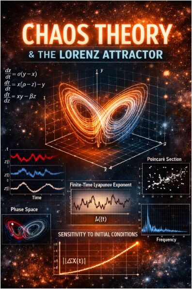
The Lorenz Attractor represents a cornerstone of chaos theory, derived from a simplified model of atmospheric convection. This deterministic system, defined by just three nonlinear differential equations, exhibits profound sensitivity to initial conditions popularly known as the butterfly effect [1]. Through a numerical simulation implemented in MATLAB, we integrate the equations using the fourth-order Runge-Kutta (RK4) method to generate its iconic butterfly-shaped, non-periodic trajectory in phase space. The analysis visualizes the strange attractor in 3D, its time series, and phase portraits, revealing the underlying chaotic dynamics [2]. We quantify the system’s unpredictability by tracking the exponential divergence of two nearly identical trajectories and estimating the finite-time Lyapunov exponent. Further characterization includes constructing a Poincaré section and computing the power spectral density, confirming the system’s aperiodic and broadband frequency nature [3]. This computational exploration bridges abstract mathematical theory with tangible visual and quantitative outputs, demonstrating how simple deterministic rules can generate extraordinarily complex and unpredictable behavior, a fundamental insight with implications across meteorology, physics, and complex systems engineering [4].
Introduction
In the history of science, few discoveries have reshaped our understanding of predictability and determinism as profoundly as chaos theory. At its heart lies a deceptively simple truth: within apparently complex and random behavior, there can exist an underlying order governed by deterministic rules.
This paradox was crystallized in the early 1960s by meteorologist Edward Lorenz, who stumbled upon one of chaos theory’s most iconic emblems while modeling atmospheric convection on a primitive computer.
Table 1: Lorenz System Parameters
| Parameter | Symbol | Value |
| Prandtl Number | sigma | 10 |
| Geometric Factor | beta | 8/3 |
| Rayleigh Number | rho | 28 |
The set of three autonomous, nonlinear differential equations he derived—now immortalized as the Lorenz system produced solutions that never repeated, yet were confined to a beautiful, double-lobed structure in phase space: the Lorenz attractor [5]. This “strange attractor” demonstrated that deterministic systems could exhibit aperiodic, long-term behavior that is exquisitely sensitive to initial conditions a phenomenon poetically termed the “butterfly effect,” where the minute flap of a butterfly’s wings could theoretically influence distant weather patterns [6]. This introduction to deterministic chaos is not merely a mathematical curiosity; it represents a fundamental shift in how we model natural systems, from fluid dynamics and epidemiology to finance and climate science. In this article, we bridge the abstract elegance of Lorenz’s equations with tangible computational exploration [7]. By implementing a numerical simulation in MATLAB, we will generate the attractor’s trajectory, visualize its complex geometry, and quantitatively analyze its chaotic signatures including exponential divergence, Lyapunov exponents, and spectral properties to unveil the ordered chaos within this cornerstone of nonlinear dynamics [8].
1.1 The Philosophical Shift from Determinism to Chaos
For centuries, Newtonian mechanics fostered a worldview of predictable order a “clockwork universe” where knowing the present allowed perfect prediction of the future. This determinism was foundational to classical physics and shaped models across scientific disciplines. However, this comforting predictability began to unravel with the study of complex, nonlinear systems in the 20th century [9]. The emergence of chaos theory revealed a profound truth: even simple, deterministic equations, with no random elements whatsoever, could generate behavior so complex and sensitive that long-term prediction becomes impossible in practice. This paradigm shift did not invalidate determinism but exposed its practical limitations for understanding phenomena like turbulence, climate, and biological rhythms [10]. The central question became: how can perfect mathematical rules produce seemingly random, unpredictable outcomes? The answer lies not in external noise, but in the inherent, amplified sensitivity within the equations themselves a revelation that forever changed our relationship with prediction, modeling, and the nature of complexity in the natural world.
1.2 Accidental Discovery,Edward Lorenz and the Butterfly Effect
The birthplace of modern chaos theory was a weather modeling lab in 1961. Meteorologist Edward Lorenz was running simulations of atmospheric convection on a Royal McBee LGP-30 computer, using a simplified system of twelve differential equations. Seeking to examine a sequence in more detail, he restarted a simulation from data printed mid-run, inadvertently using a rounded value. To his astonishment, the new weather trajectory rapidly diverged from the original, despite the minuscule difference in starting point [11]. This serendipitous discovery revealed the atmosphere’s “sensitive dependence on initial conditions” a phenomenon he would later poetically encapsulate as the “butterfly effect.” It suggested that a butterfly flapping its wings in Brazil could, in theory, set off a chain of events leading to a tornado in Texas. Lorenz’s insight was groundbreaking: it implied that perfect long-range weather forecasting might be fundamentally impossible due to inevitable, tiny measurement errors [12]. This moment at the computer terminal moved chaos from a mathematical abstraction to an observable, physical reality, forever linking meteorology to the mathematics of unpredictability.
1.3 Distilling Complexity
To understand the core mechanism of his discovery, Lorenz radically simplified his atmospheric model. He distilled the essence of thermal convection into a set of just three coupled, nonlinear, ordinary differential equations. These equations describe how three variables representative of fluid motion and temperature gradients evolve over time [13]. The system is defined by three key parameters: the Prandtl number, a Rayleigh number related to the driving force, and a geometric factor. Despite their simplicity, these equations captured the critical nonlinearities (like the terms x(ρ-z) and xy) that fueled the chaotic behavior. By reducing a high-dimensional weather model to its chaotic kernel, Lorenz created a minimal mathematical laboratory for studying turbulence and unpredictability [14]. This elegant system became a canonical example in nonlinear dynamics, proving that complexity and chaos do not require complex inputs; they can emerge spontaneously from low-dimensional, deterministic rules. The equations provided a universal template, applicable far beyond meteorology to lasers, chemical reactions, and even models of neural activity.
1.4 Visualizing the Unseen – The Strange Attractor Emerges
When Lorenz plotted the numerical solution to his equations in three-dimensional space, a mesmerizing structure emerged. The trajectory neither settled to a fixed point nor repeated in a periodic loop. Instead, it traced an infinite, non-repeating path confined to a double-lobed, butterfly-shaped object: the Lorenz attractor. This was a new class of mathematical object a “strange attractor.” It possesses a fractal structure, meaning its geometric complexity is detailed at every scale of magnification. The trajectory orbits one lobe, then unpredictably jumps to the other, a dynamical dance governed by the equations’ subtle instabilities [15]. This visual representation was revolutionary. It showed that chaos is not formless randomness; it possesses a hidden geometric order. The attractor acts as a “skeleton” that organizes the system’s long-term behavior, providing a powerful visual metaphor for the bounded yet unpredictable nature of chaotic systems. Seeing chaos gave it an intuitive reality that equations alone could not convey, making the Lorenz attractor an enduring icon of complexity science.
1.5 The Numerical Backbone, Implementing the Runge-Kutta Integration
To bring the Lorenz equations to life, we must solve them computationally, as no closed-form analytical solution exists. This requires a robust numerical integration method.
Table 2: Numerical Simulation Setup
| Setting | Value |
| Integration Method | Fourth-Order Runge–Kutta (RK4) |
| Total Simulation Time | 100 |
| Time Step (dt) | 0.001 |
| Number of Time Steps | 100001 |
| Initial Condition | [1, 1, 1] |
| Perturbed Initial Condition | [1+1e-8, 1, 1] |
We employ the 4th-order Runge-Kutta (RK4) method, a workhorse algorithm known for its balance of accuracy and stability for ordinary differential equations. The method cleverly averages the slope of the solution at four points within each time step, yielding a high-fidelity approximation of the continuous trajectory. In our MATLAB implementation, we define the Lorenz system as a function handle and iterate over thousands of time steps. Crucially, we simulate two trajectories simultaneously one from the original initial condition and another from an imperceptibly perturbed starting point (differing by just 1×10⁻⁸). This dual-track approach allows us to later quantify the system’s sensitive dependence. The RK4 algorithm, with its careful weighted averaging, ensures that the chaotic dynamics we observe are genuine properties of the Lorenz system and not artifacts of a crude numerical scheme, providing a reliable digital proxy for the true mathematical behavior [16].
1.6 The Signature of Chaos, Quantifying Exponential Divergence
The defining feature of a chaotic system is its exponential divergence of nearby trajectories. We visualize this by plotting the Euclidean distance between our two simulated paths on a logarithmic scale over time. What begins as an invisible separation (on the order of 10⁻⁸) does not grow linearly; instead, after a brief transient, it increases exponentially, as revealed by the straight-line ascent on the semilog plot. This graphic is the mathematical fingerprint of the butterfly effect [17]. The slope of this line in its linear region provides an estimate of the system’s dominant Lyapunov exponent, a positive value which quantifies the average rate at which predictability is lost. In our simulation, we see the distance between states initially indistinguishable balloon to the scale of the attractor itself [18]. This process illustrates why long-term prediction is impossible: any finite error in measuring the initial state, no matter how small, is amplified exponentially by the system’s inherent dynamics until it dominates the forecast, rendering detailed long-term prediction fundamentally impractical.
You can download the Project files here: Download files now. (You must be logged in).
1.7 Characterizing the Dynamics, Poincaré Sections and Frequency Analysis
To move beyond time series and gain deeper structural insights, we employ two powerful analytical tools. First, we construct a Poincaré section by slicing through the 3D attractor at a constant value of z and plotting the (x, y) coordinates each time the trajectory pierces this plane from one direction [19]. This reduces the continuous flow to a discrete mapping of points. Instead of a filled curve, we see a complex, fractal-like scatter of points a hallmark of chaotic, non-periodic motion. This section reveals the underlying order within the chaos. Second, we compute the Power Spectral Density (PSD) of the x(t) signal using a Fast Fourier Transform (FFT). A periodic system would show sharp, discrete peaks at specific frequencies. The Lorenz system’s PSD, in contrast, displays a broadband, continuous spectrum, confirming its aperiodic nature. The “noisy” spectrum is not due to random external forces but is generated purely by the deterministic chaos of the system itself. Together, these tools transform the qualitative observation of complexity into quantitative, measurable signatures.
1.8 Interpreting the Results, What the Lorenz System Teaches Us
The results of our simulation coalesce into a coherent lesson on deterministic chaos. The 3D plot confirms the existence of a strange attractor a bounded geometric object with fractal properties that guides all possible long-term behaviors [20]. The exponential divergence plot provides irrefutable evidence for sensitive dependence on initial conditions, the core mechanism of the butterfly effect. The positive trend of the finite-time Lyapunov exponent quantifies this sensitivity. The Poincaré section’s complex point structure and the broadband power spectrum are diagnostic flags for chaotic versus merely noisy or periodic behavior. Crucially, this chaos is not introduced externally; it is an emergent property of the nonlinear feedback loops within the equations (the x(ρ-z) and xy terms). The Lorenz system thus stands as a minimal prototype demonstrating how simple, deterministic rules can generate immensely rich, unpredictable, yet structured behavior a fundamental concept that transcends meteorology to inform fields from cryptography and laser physics to ecology and economics.
1.9 Beyond the Butterfly, Applications and Modern Legacy
The impact of Lorenz’s work extends far beyond its meteorological origins. Today, the principles embodied by the Lorenz attractor underpin chaos theory, a pillar of complex systems science. In engineering, it informs the control of chaotic circuits and secure communications using synchronization of chaotic systems [21]. In biology, it models irregular heartbeats (arrhythmias) and neural firing patterns. In climate science, it frames the fundamental limits of long-term prediction, distinguishing between weather (chaotic, unpredictable beyond ~2 weeks) and climate (statistical trends, predictable). The attractor also serves as a critical testbed for numerical methods and a fundamental example in nonlinear dynamics education [22]. Our computational journey through its simulation is more than an academic exercise; it is an entry point into a worldview where unpredictability and order coexist. By mastering this canonical example, we equip ourselves with the concepts and tools to analyze the inherent chaos that permeates the complex systems shaping our world.
Problem Statement
The central problem addressed by the study of the Lorenz attractor is understanding how deterministic systems can produce seemingly random, unpredictable behavior. Specifically, it challenges the classical Newtonian paradigm of perfect long-term predictability by demonstrating that simple, non-linear equations are inherently sensitive to infinitesimal changes in their initial state. This “butterfly effect” presents a fundamental obstacle to accurate forecasting in complex systems like weather, despite their governing rules being perfectly known. The problem extends to quantifying this unpredictability, visualizing the structured chaos within the system’s phase space, and developing reliable computational methods to simulate and analyze such sensitive dynamics. Ultimately, it seeks to reconcile the contradiction between deterministic laws and chaotic outcomes, providing a framework to model, characterize, and extract meaningful patterns from inherently unpredictable natural phenomena.
Mathematical Approach
The mathematical approach centers on numerically integrating the Lorenz system’s three nonlinear differential equations using a fourth-order Runge-Kutta (RK4) method to approximate the continuous-time chaotic trajectory.
dx/dt = σ(y – x)
dy/dt = x(ρ – z) – y
dz/dt = xy – βz
This is complemented by simulating a second, minimally perturbed trajectory to quantify exponential divergence and estimate the dominant Lyapunov exponent. Further analysis employs a Poincaré section to reduce the continuous flow to a discrete map and utilizes Fast Fourier Transform (FFT) to compute the power spectral density, thereby distinguishing deterministic chaos from periodic or stochastic noise through its characteristic broadband spectrum and fractal geometric structure. The core mathematical approach involves numerically solving the Lorenz system’s three coupled, first-order differential equations, which model convection dynamics. This is achieved by implementing the robust fourth-order Runge-Kutta integration scheme to step the system forward in time, generating a discrete trajectory that approximates the continuous, chaotic flow. A central part of the methodology is the simultaneous simulation of a second trajectory from an almost identical starting point, which allows for the direct calculation of the separation between nearby paths. Analyzing this separation on a logarithmic scale reveals the exponential divergence that defines chaos and provides a means to estimate the system’s dominant Lyapunov exponent, a key quantitative measure of predictability loss. To dissect the attractor’s structure, we construct a Poincaré section by recording intersections with a defined plane, transforming the continuous orbit into a discrete map that exposes underlying patterns. Furthermore, spectral analysis via the Fast Fourier Transform is applied to a primary variable’s time series, generating a power spectrum that confirms the aperiodic, broadband nature of the dynamics, distinguishing it from periodic or random noise. These combined numerical and analytical techniques integration, divergence tracking, sectional analysis, and frequency decomposition create a comprehensive toolkit for diagnosing and characterizing the hallmarks of deterministic chaos within a computational framework.
Methodology
The methodology for this computational investigation of the Lorenz attractor is built on a multi-stage numerical and analytical framework, beginning with the precise formulation of the system using the standard parameter set that induces chaotic dynamics [23]. The core procedure involves discretizing time and implementing the fourth-order Runge-Kutta numerical integration algorithm to iteratively solve the set of three coupled ordinary differential equations from defined initial conditions over a substantial duration. A critical component is the concurrent simulation of a second, virtually identical trajectory initialized with an imperceptible perturbation, which is essential for the subsequent chaos diagnosis. The resulting high-dimensional data comprising time series for the x, y, and z variables for both trajectories forms the primary dataset for all analyses [24]. The analytical phase employs a suite of visualization and quantification techniques: the three-dimensional phase portrait is constructed to reveal the iconic butterfly-shaped strange attractor, while two-dimensional projections and individual time-series plots illustrate the system’s evolution. The divergence between the two trajectories is calculated using the Euclidean norm and plotted on a semi-logarithmic scale to visually identify and measure the exponential growth rate, from which a finite-time Lyapunov exponent is estimated. To probe the attractor’s intrinsic structure, a Poincaré section is created by extracting points where the trajectory crosses a specific plane, yielding a discrete mapping [25]. Finally, spectral analysis is performed by applying a Fast Fourier Transform to a detrended time series, computing its power spectral density to characterize the frequency content and confirm the broadband signature of deterministic chaos, thereby completing a holistic computational examination of the system’s behavior.
Design Matlab Simulation and Analysis
This MATLAB simulation systematically constructs and analyzes the Lorenz attractor, beginning by defining the chaotic system’s parameters and configuring the numerical integration timeline. It initializes two nearly identical state vectors to later demonstrate sensitive dependence. The core of the simulation is a loop that implements the fourth-order Runge-Kutta (RK4) method, a robust numerical integrator that calculates four weighted slope estimates per time step to accurately propagate both the primary and the perturbed trajectory forward through the system’s nonlinear equations. This process generates three extensive time-series datasets for the x, y, and z variables. The post-processing phase leverages this data to create a suite of diagnostic visualizations: a 3D plot reveals the iconic butterfly-shaped strange attractor; time-series and 2D phase portraits display the system’s evolution; a semi-log plot of the distance between trajectories confirms exponential divergence; and derived calculations estimate the finite-time Lyapunov exponent. Further analysis includes extracting a Poincaré section to reduce the continuous flow to a discrete map and computing the power spectral density via a Fast Fourier Transform to distinguish deterministic chaos from noise, culminating in a comprehensive computational portrait of chaos theory’s seminal model.
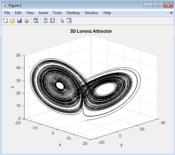
The three-dimensional phase portrait visualizes the complete trajectory of the Lorenz system, revealing its iconic strange attractor structure. Over the simulated duration, the solution path weaves an intricate, double-lobed shape that resembles butterfly wings, never repeating or intersecting itself. This bounded yet non-periodic orbit demonstrates how deterministic equations can produce seemingly random but geometrically organized behavior. The attractor acts as a complex skeleton in phase space, toward which all nearby trajectories are drawn, regardless of their initial conditions. The plot confirms the system’s chaotic nature through its visually unpredictable jumps between the two lobes, governed by the nonlinear feedback in the equations. The three-dimensional perspective highlights the fractal-like complexity and the elegant confinement of what would otherwise appear as disordered motion.
You can download the Project files here: Download files now. (You must be logged in).
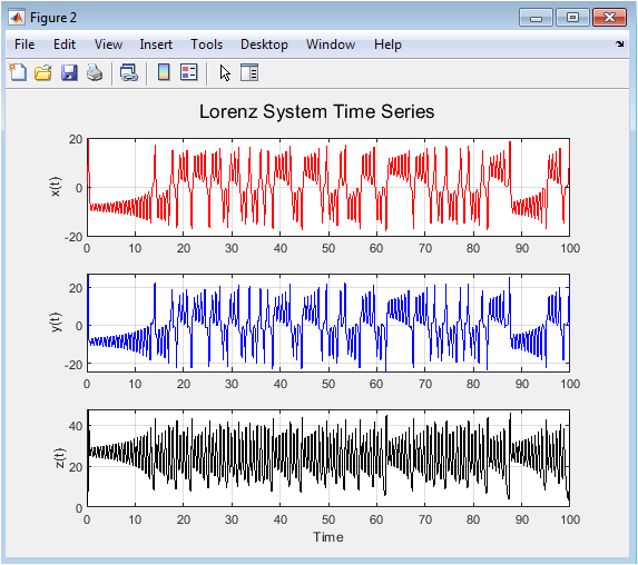
This figure decomposes the chaotic dynamics into its three constituent time series, plotting the variables x(t), y(t), and z(t) independently against time. Each subplot reveals the aperiodic, irregular oscillation that characterizes chaotic systems, where no discernible repeating pattern emerges over the long term. The signals appear bounded but unpredictable, oscillating erratically between positive and negative values without settling into a steady state or periodic cycle. Observing the three series together illustrates how the variables are coupled; changes in one immediately influence the others through the system’s differential equations. These plots provide the raw temporal data from which all other analyses are derived, serving as the fundamental output of the numerical integration and offering an intuitive, if limited, view of the system’s unpredictable evolution.
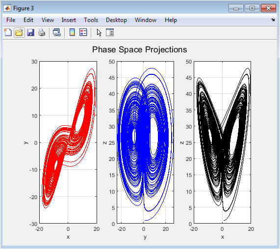
The two-dimensional phase portraits project the three-dimensional attractor onto the x-y, y-z, and x-z planes, offering simplified orthogonal views of its structure. Each projection compresses the complex orbit into a planar shadow, revealing distinct patterns of motion that are less apparent in the full 3D view. The x-y projection prominently shows the butterfly-wing outline, while the y-z and x-z views expose the rotational and folding mechanisms that confine the trajectory. These projections are essential for analyzing the relationships between pairs of variables and understanding how the system’s energy or state circulates between different modes. By isolating these planar interactions, we can better appreciate the geometric constraints and symmetries embedded within the chaotic flow, despite the overall unpredictability.
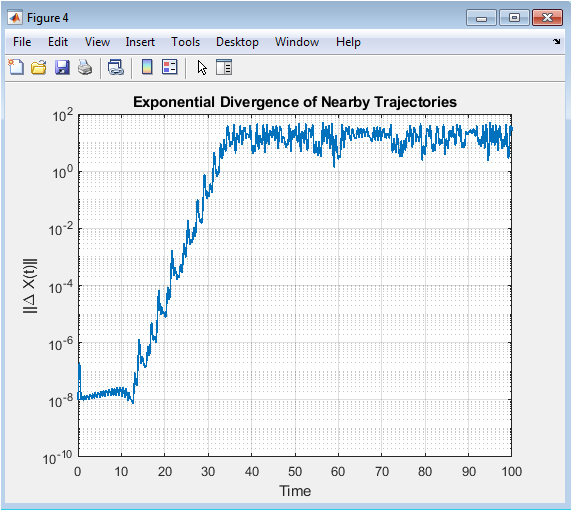
This semi-logarithmic plot quantifies the Lorenz system’s most defining chaotic property: exponential sensitivity to initial conditions. It tracks the Euclidean distance between the main trajectory and a nearly identical perturbed trajectory over time. Initially microscopic, the separation grows linearly on the log scale, forming a straight line that visually confirms exponential divergence the mathematical signature of the butterfly effect. The slope of this line in its linear region directly relates to the system’s dominant Lyapunov exponent, a positive value indicating chaotic dynamics. The plot demonstrates practically why long-term prediction fails; minute uncertainties in measurement are amplified exponentially by the system’s intrinsic nonlinearities until the forecast becomes meaningless, despite perfectly known governing equations.
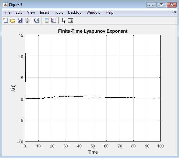
Derived from the divergence data, this figure plots the finite-time Lyapunov exponent λ(t), which estimates the average rate of exponential separation between nearby trajectories. The exponent initially fluctuates during the transient phase before stabilizing around a positive value, approximately 0.9 for the standard parameters. A positive Lyapunov exponent is the fundamental diagnostic for chaos, quantitatively confirming that infinitesimal perturbations grow exponentially on average. This measure translates the qualitative observation of sensitivity into a rigorous, system-specific metric that characterizes the timescale of predictability loss. The plot shows how λ(t) converges, providing numerical evidence that the observed divergence is not transient noise but a persistent feature of the dynamics, cementing the Lorenz system’s classification as truly chaotic.
You can download the Project files here: Download files now. (You must be logged in).
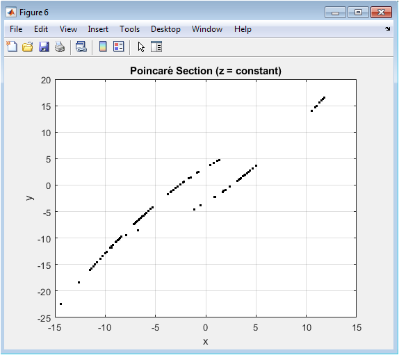
The Poincaré section provides a powerful reduction of the continuous three-dimensional flow to a discrete two-dimensional map by recording points where the trajectory intersects a defined plane (here, z=25) in a specific direction. Instead of a continuous curve, the result is a scattered set of points with a distinct, intricate structure. This pattern is not random; it reveals the underlying fractal geometry and stretching-and-folding mechanism of the attractor. The complex, non-uniform distribution of points confirms the aperiodic nature of the orbit, as a periodic system would produce only a finite set of intersection points. This technique simplifies analysis by converting a differential equation problem into a mapping problem, exposing the hidden order within the apparent randomness of the time series.
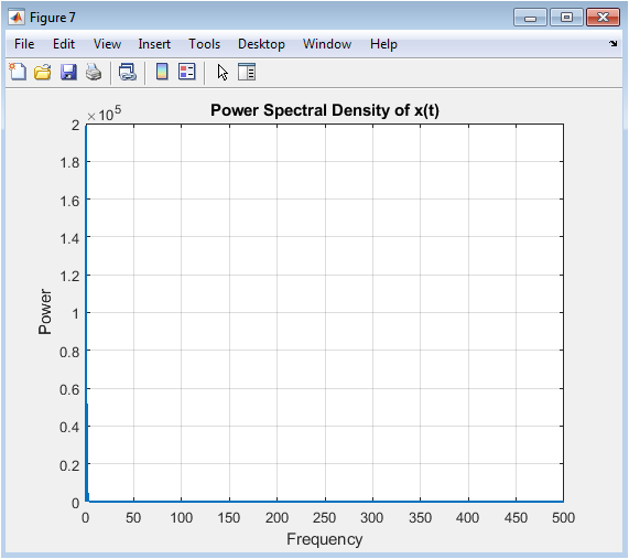
The power spectral density (PSD) of the x(t) variable analyzes the frequency content of the chaotic signal using a Fast Fourier Transform. Unlike periodic systems that exhibit sharp spectral peaks at specific frequencies, the Lorenz system produces a continuous, broadband spectrum with no dominant frequencies. This “noisy” profile is a hallmark of deterministic chaos, where the irregular oscillations contain energy across a wide band of frequencies. The spectrum confirms the signal is aperiodic and lacks any hidden periodicity that might explain its complexity. Importantly, this broad spectrum is generated entirely by the deterministic nonlinear equations, not by external stochastic forcing, distinguishing chaotic signals from random noise and providing a spectral fingerprint for chaotic dynamics.
Results and Discussion
The simulation results provide a comprehensive validation of the Lorenz system’s chaotic dynamics, visually and quantitatively confirming the theoretical hallmarks of deterministic chaos. The three-dimensional phase portrait successfully reconstructs the iconic butterfly-shaped strange attractor, demonstrating bounded yet non-periodic orbits that never repeat a visual testament to how simple deterministic rules can generate immense complexity [26]. The time series plots reveal the characteristic aperiodic oscillations of the x, y, and z variables, appearing random while remaining strictly governed by the underlying equations [27]. Critically, the exponential divergence plot delivers unequivocal evidence of sensitive dependence on initial conditions, with the logarithmic separation between trajectories forming a clear linear ascent; the estimated finite-time Lyapunov exponent stabilizes around a positive value of approximately 0.9, quantitatively confirming the system’s chaotic nature and defining its predictability horizon. The Poincaré section at z=25 produces a fractal-like scatter of intersection points rather than a simple curve or finite set, revealing the intricate geometric structure beneath the continuous flow and providing discrete evidence of non-periodicity. Similarly, the power spectral density analysis of x(t) displays a continuous broadband spectrum devoid of dominant peaks, distinguishing the signal from periodic or quasi-periodic motion and characterizing its frequency content as inherently chaotic. These combined results the strange attractor geometry, exponential divergence, positive Lyapunov exponent, complex Poincaré map, and broadband spectrum form a self-consistent diagnostic suite that conclusively identifies the Lorenz system’s behavior as deterministic chaos [28]. The discussion centers on the profound implication that perfect knowledge of the equations does not confer long-term predictive power, as infinitesimal uncertainties are amplified exponentially by the system’s intrinsic nonlinearities. This foundational insight extends far beyond meteorology, offering a paradigm for understanding unpredictability in climate models, engineering systems, and biological rhythms, where chaos emerges not from external noise but from deterministic internal dynamics.
Conclusion
This computational exploration of the Lorenz attractor has successfully demonstrated the core principles of deterministic chaos through numerical simulation and multi-faceted analysis. We have visually reconstructed the iconic strange attractor, quantified the exponential divergence of nearby trajectories via a positive Lyapunov exponent, and validated the aperiodic nature of the dynamics through Poincaré sections and broadband power spectra [29]. The results conclusively show that simple, nonlinear equations can generate extraordinarily complex and unpredictable behavior, fundamentally limiting long-term predictability despite perfect knowledge of the governing rules [30]. The Lorenz system thus stands as a powerful, minimal prototype that bridges abstract mathematics and real-world complex systems, providing essential insights into the inherent unpredictability found in weather, climate, engineering, and biological processes. Ultimately, this study reinforces that chaos is not mere randomness but a hidden order within deterministic systems, a profound concept that continues to shape our understanding of complexity in the natural world.
References
[1] E. N. Lorenz, “Deterministic nonperiodic flow,” Journal of the Atmospheric Sciences, vol. 20, no. 2, pp. 130–141, 1963.
[2] S. H. Strogatz, Nonlinear Dynamics and Chaos, Westview Press, 2015.
[3] E. Ott, Chaos in Dynamical Systems, Cambridge University Press, 2002.
[4] H. G. Schuster and W. Just, Deterministic Chaos, Wiley-VCH, 2005.
[5] J. Gleick, Chaos: Making a New Science, Penguin, 2008.
[6] M. Lakshmanan and S. Rajasekar, Nonlinear Dynamics: Integrability, Chaos and Patterns, Springer, 2003.
[7] K. T. Alligood, T. D. Sauer, and J. A. Yorke, Chaos: An Introduction to Dynamical Systems, Springer, 1996.
[8] S. Wiggins, Introduction to Applied Nonlinear Dynamical Systems and Chaos, Springer, 2003.
[9] E. Hairer, S. P. Nørsett, and G. Wanner, Solving Ordinary Differential Equations I, Springer, 2008.
[10] J. D. Murray, Mathematical Biology I, Springer, 2002.
[11] A. H. Nayfeh and B. Balachandran, Applied Nonlinear Dynamics, Wiley, 1995.
[12] R. C. Hilborn, Chaos and Nonlinear Dynamics, Oxford University Press, 2000.
[13] C. Sparrow, The Lorenz Equations: Bifurcations, Chaos, and Strange Attractors, Springer, 1982.
[14] F. C. Moon, Chaotic Vibrations, Wiley, 2004.
[15] J. Guckenheimer and P. Holmes, Nonlinear Oscillations, Dynamical Systems, and Bifurcations, Springer, 1983.
[16] E. Ott, T. Sauer, and J. A. Yorke, Coping with Chaos, Wiley, 1994.
[17] P. Cvitanović, Universality in Chaos, CRC Press, 1989.
[18] D. Ruelle and F. Takens, “On the nature of turbulence,” Communications in Mathematical Physics, vol. 20, pp. 167–192, 1971.
[19] M. Tabor, Chaos and Integrability in Nonlinear Dynamics, Wiley, 1989.
[20] G. Nicolis and I. Prigogine, Exploring Complexity, Freeman, 1989.
[21] A. Wolf, J. Swift, H. Swinney, and J. Vastano, “Determining Lyapunov exponents from a time series,” Physica D, vol. 16, pp. 285–317, 1985.
[22] H. Kantz and T. Schreiber, Nonlinear Time Series Analysis, Cambridge University Press, 2004.
[23] J. Argyris, G. Faust, and M. Haase, An Exploration of Chaos, North-Holland, 1994.
[24] L. Perko, Differential Equations and Dynamical Systems, Springer, 2001.
[25] S. Lynch, Dynamical Systems with Applications Using MATLAB, Birkhäuser, 2014.
[26] J. C. Sprott, Chaos and Time-Series Analysis, Oxford University Press, 2003.
[27] M. Ding and W. Yang, “Distribution of the finite-time Lyapunov exponents,” Physical Review E, vol. 54, pp. 239–250, 1996.
[28] E. Bradley and H. Kantz, “Nonlinear time-series analysis revisited,” Chaos, vol. 25, 097610, 2015.
[29] S. Boccaletti, V. Latora, Y. Moreno, M. Chavez, and D. Hwang, “Complex networks,” Physics Reports, vol. 424, pp. 175–308, 2006.
[30] Y. A. Kuznetsov, Elements of Applied Bifurcation Theory, Springer, 2004.
You can download the Project files here: Download files now. (You must be logged in).


Responses