

Simulation of Thermodynamic Efficiency in Combined-Cycle Power Plants Using OpenModelica
Author: Waqas Javaid
Abstract
Renewable energy has already proved to be a reliable and economic source of energy production. However, in 2018 renewable energy only accounted for 12.7% of the total energy produced within the United States; this makes it a relatively small contributor when compared to natural gas, petroleum, and coal. The Thermal Sciences Group at the National Renewable Energy Laboratory (NREL) aims to change this statistic by the research and innovation on the forefront of renewable energy technologies. The software OpenModelica is poised as a potential tool to help NREL’s research team model and design future complex systems prior to prototyping and implementation. However, there is little information known about this software (i.e., ease of modeling, reliability of models, and scope of application). A model study of a combined-cycle power plant has been conducted in order to validate the opensource software, OpenModelica.
The model study is intended to describe a combined-cycle power plant with a constant pressure heat recovery steam generator, and to analyze the combined-cycle effectiveness to produce a prescribed power load of 100 [MW]. The exploration and developmental work produced from this OpenModelica case study will open the knowledge base for broad implementation of this software in various application scenarios.
1. Introduction
In today’s age, most complex engineered systems are built and designed with computational modeling software. Designing, fabricating, and maintaining a complex system by hand can be considered redundant. It can be very expensive and can lead to a misuse of resources if the system does not function as intended. Modeling and simulation activities play a key role in the design phase and performance optimization of complex energy processes. It is also expected that they will play a significant role in the future for power plant maintenance and operation 1. We have chosen the software OpenModelica to serve as the computational modeling tool to design and simulate a thermal energy storage system.
Modelica is an Equation-Based Object-Oriented (EOO) modeling language that is open source and managed by the Modelica Association. The Modelica language was intended for users to be able to describe engineering components and systems. The language’s declarative, acausal nature provides a wide spectrum of modeling ease for all backgrounds. The Modelica language needs a specific programming environment for it to be programmed in, which increases the complexity of using this software [2].
In this study, OpenModelica was chosen to be the modeling environment for the Modelica language. This choice was justified because it is an open source software and is supported by the Open Source Modelica Consortium (OSMC). Being supported and affiliated with the OSMC, there are valuable modules provided for its modeling environment that make the modeling process more user-friendly [2].
The modeling process starts with the OMNotebook. The OMNotebook is an interactive Modelica language learning tool that provides users with a strong understanding of the language basics through coding tutorials. The learning approach is supported by hierarchical text documents composed of chapters and sections [3]. All aspects of the EOO language were explored to help enable future users who wish to model using OpenModelica’s OMEdit module.
OMEdit, a graphical user interface (GUI) module, is the main workspace within the OpenModelica modeling environment. Within this GUI, users have the option of building models from either a code-based approach, a visual-based approach, and even the option to alternate between both approaches. The code-based approach entails that the user will be working within the “Text View” of OMEdit and building their model of interest by writing in Modelica’s EOO language. The visual-based approach entails that the user will be working within the “Diagram View” of OMEdit and building their model of interest by virtually connecting block-diagram components. Whether the model is being built within the “Text View” or the “Diagram View”, the modeling approach can be switched back and forth because both “views” represent the same model. Once a system model has been completed, OMEdit is available for further model support. OMEdit has the Debugger that is intended to help their users check their model’s stability and help solve model errors when they arise. For models that are “square” in size (equal number of equations and variables within the model) and can flatten (instantiate), OMEdit provides a Plotting tool to study a system’s parameters under a controlled virtual simulation. Modelica’s declarative, acausal EOO language allows users to change/vary a model’s system parameters to explore alternative capabilities or failures of a system without having to change the computational code supporting the model. This is an advantage over other modeling software because the computational instructions change as one changes the input parameters. This gives the Plotting tool within the OMEdit GUI a lot of power to explore system capabilities that are not feasible within reality. OMEdit is the paramount module within OpenModelica because it gives users the capability to model, debug, and plot model results all within the same GUI.
The final module to be recognized is the Modelica Standard Library (MSL) that users can access within the OMEdit GUI. The MSL is an open source library from the Modelica Association to model mechanical (1D/3D), electrical (analog, digital, machines), magnetic, thermal, fluid, control systems and hierarchical state machines [4]. The MSL is a robust tool that highlights the wide range of Modelica’s EOO language applications. This component library provides the ability for the re-use and exchange of models in a standardized format. Having to re-write computational code for models in different applications/scenarios is a common issue associated with traditional modeling languages 5. Modelica’s EOO language allows users to have the ability to write a component’s code once and then re-use the component for a wide range of applications. Building computational models is made simple because each component is ready to be dragged and dropped into the model-building workspace.
NREL has an ever increasing need to be able to model and study complex dynamic systems of interest in an easy and variable method. Building the real systems under investigation can be very costly, time-consuming, and sometimes they have still yet to exist [6]. The software OpenModelica serves as an ideal tool that is free and flexible across a wide array of applications. It is in NREL’s best interest to use OpenModelica for the modeling of complex dynamic systems.
You can download the Project files here: Download files now. (You must be logged in).
2. EOO Fundamentals
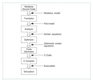
To understand the significance of Modelica’s Equation-Based Object-Oriented (EOO) language, it is important to understand what it is not. There are roughly two kinds of modeling languages: imperative languages and equational languages. Imperative languages like Fortran, C, C++, Java, etc. are used for imperative programming which consists of writing explicit algorithms that compute model’s equations [7]. This requires extensive backend work for the user who must manually calculate and solve for the variable of interest in order to give computing instructions that compute the numerical solution for the equation [7]. It is much more appropriate to perform this task automatically by using an equational modeling language. The equational language lets the user express the model’s mathematical equations as they are without further simplification into an algorithm. This is called acausal modeling. Users can simply insert the governing equations of a specific model directly from the textbook, without having to solve for any variables of interest. Here, equations do not specify which variables are inputs and which are outputs, whereas in assignment statements variables on the left-hand side are always outputs (results) and variables on the right-hand side are always inputs [8]. As seen in Figure 1, the Modelica compilers automatically determine the computational solution by translating equational models into imperative programs, which are in turn compiled with regular compilers (C, C++, Fortrans, etc.) to produce executable code [7] [9].

- Figure 1. OpenModelica model compilation logic flow [10]
Much of the power of modeling with Modelica comes from the ease of reusing model classes. As an equation-based modeling language, Modelica has been designed to allow tools to automatically generate efficient simulation code with the important objective of facilitating exchange and reuse of models, model libraries, and simulation specifications [9]. Modelica’s EOO language supports this standardized exchange of information for all components. Composing a model from existing Modelica libraries targeting different domains, such as electrical and mechanical, is as easy as dragging and dropping model components from the libraries onto a diagram and connecting the models together [9]. The automatic source code generated is used to facilitate the flow of information from one component to another. This autonomous action can be attributed to the equations that govern all the models; the conservation of mass, momentum, and energy equations. The fundamental conservation equations can apply to all components of all domains. As seen in Figure 2, components within a model act as control-volumes, where anything that comes into the component (i.e. start value(s), end value(s), component parameters, etc.) will come back out and will be fed into the next component in sequence. Modelica’s EOO language is what gives the OpenModelica modeling environment it’s unique flexibility and robustness as a software modeling application.

- Figure 2. Visual representation of “acausal” modeling between two components [11]

3. Model Building Overview
For complex dynamic systems, there can be multiple sub-systems with each of their own respective functions. For multiple sub-systems to be working together harmoniously in an EOO modeling environment, the components within the model need to facilitate a seamless exchange of information with one another. This is accomplished by applying the fundamental continuity equations to components which act as control volumes [1].
A combined-cycle power plant model should incorporate the fundamental sciences occurring within the system: thermodynamics and heat transfer. The ThermoPower Library, MSL, and many other OpenModelica component libraries apply the relevant, fundamental continuity equations to facilitate information exchanges between interconnected components. The continuity equations can describe the physical interactions that occur between the thermodynamic cycles and interacting fluids within the combined-cycle power plant model. The mass, momentum, and energy continuity equations below have been adapted to describe the thermodynamic and heat transfer interactions that occur within a combined-cycle power plant.
3.1. Mass balance equation
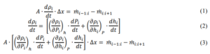
The mass balance equations for any mixture can be obtained by the summation of partial derivatives with respect to enthalpy and pressure of the flow. The mass balance equation in each cell is given by Equation 1, which is further simplified to Equation 3.
3.2. Momentum balance equation
The momentum balance equations for any mixture can be obtained by the summation of pressure changes throughout a cell as well as the losses associated with the flow. The momentum balance equations in each cell is given by Equation 3 supplemented by Equations 4-8.
![]()
The change of pressure due to acceleration can be given by Equation 4.
![]()
The change in pressure due to friction can be given by Equation 5.
![]()
The change in pressure due to gravity can be given by Equation 6.
![]()
By default, the flow is considered turbulent (Reynolds number Re > 2300). The COLEBROOK correlation is used in Equation 7.
![]()
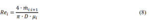
The Reynolds number of a fluid flowing through a cell can be given by Equation 8.
3.3 Energy balance equation
The energy balance equation for any mixture can be obtained by the summation of enthalpy changes associated with the mass flow rates entering and leaving a component’s cell. The energy balance equation in each cell is given by Equation 9 and further simplified to Equation 11.
4. Modeling Results
This section outlines the different types of system models produced, their ability to function, and the steps taken to parametrize the model.
4.1. Brayton-cycle model – square in size & working simulation

- Figure 3. OpenModelica Brayton-cycle model schematic of Diagram view within OMEdit
4.1.1 Brayton-cycle model assumptions
To apply the fundamental continuity equations on our system, there are some model assumptions that need to be made. For the Brayton cycle, it is assumed that it is an ideal and reversible open- cycle system. It is also assumed that the fluid throughout the system will be treated as air, the compression rate (cpr) will equal 10, and that the power produced will equal 70 [MW]. The power distribution throughout the system can be exemplified by Equation 11 below.
![]()
4.1.2 Brayton-cycle model description
The OpenModelica Brayton model consists of one compressor, one combustion chamber, one combustion turbine, one generator, one pressure source, one pressure sink, one mass flowrate regulator, two pressure drops, and several sources. The model contains one open loop, where the hot exhaust gases are expelled to the outside environment.
You can download the Project files here: Download files now. (You must be logged in).
4.1.3 Brayton-cycle thermodynamic analysis

- Figure 4. Brayton-cycle P-v diagram
Table 1. Brayton-cycle thermodynamic state analysis
State 1 | State 2 | State 3 | State 4 | |
Pressure, P [bar] | 1 | 10 | 10 | 1 |
Temperature, T [K] | 300 | 574.09 | 1400 | 787.72 |
Specific Enthalpy, h [kJ∙kg-1] | 300.19 | 579.86 | 1515.4 | 808.49 |
![]()
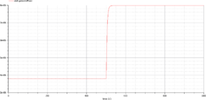
4.1.4 Brayton-cycle OpenModelica Simulation Plot

- Figure 5. OpenModelica Brayton model steady state “power generated” simulation
4.2 Rankine-cycle model – square in size & broken simulation

- Figure 6. OpenModelica Rankine-cycle model schematic of Diagram view within OMEdit
4.2.1 Rankine-cycle model assumptions
To apply the fundamental continuity equations on our system, there are some model assumptions that need to be made. For the Rankine cycle, it is assumed that it is an idea and reversible closed- cycle system. It is also assumed that the water flowing throughout the system will be treated as either a liquid, gas, or a two-phase mixture, there is constant pressure throughout the HRSG, and that the power produced will equal 30 [MW]. The power distribution throughout the system can be exemplified by equation 13 below.
![]()
4.2.2 Rankine-cycle model description
The OpenModelica Rankine model consists of three heat exchangers (1 economizer, 1 evaporator, and 1 super-heater), one steam turbine, one condenser, one pump, several sources, and one sink. The model contains one closed loop for the water/steam cycle and one open loop for the fluegas. An important feature of this model is that the thermodynamic cycle is completely closed through the condenser.
4.2.3 Rankine-cycle thermodynamic analysis

- Figure 6.1 Rankine-cycle T-s diagram
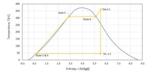
Table 2. Rankine power-cycle thermodynamic state analysis
Pressure [bar] | Temperature [K] | Specific Enthalpy [kJ∙kg–1] | Specific Entropy [kJ∙kg–1] | |
State 1 | 100 | 633.15 | 2962.10 | 6.006 |
State 2 | 0.1 | 318.96 | 1900.63 | 6.006 |
State 3 | 0.1 | 318.96 | 191.83 | 0.6493 |
State 4 | 100 | 319.60 | 203.22 | 0.6493 |
State 5 | 100 | 584.25 | 1407.60 | 3.3596 |
State 6 | 100 | 584.25 | 2724.70 | 5.6141 |
Wcycle,R = Wturbine + Wpump = 30 [MW]
30 [MW] = 𝑚̇ ∙ (h1 – h2) + 𝑚̇ ∙ (h3 – h4)
𝑚̇ = 21.5 [kg∙s-1]
(Needed for prescribed load of combined-cycle power plant)
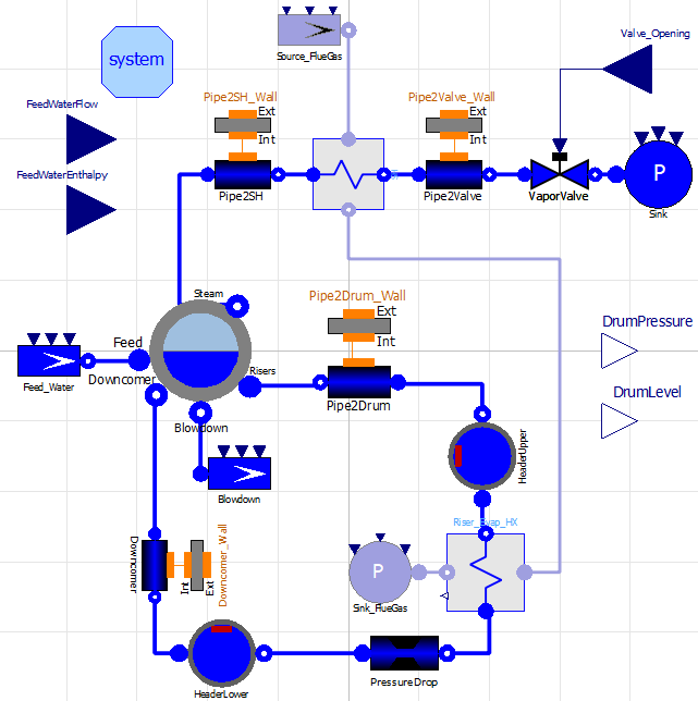
4.3. Heat Recovery Steam Generator model – square in size & broken simulation

- Figure 7. Heat Recover Steam Generator (HRSG) model schematic of Diagram view within OMEdit

4.3.1 HRSG model assumptions
To apply the fundamental continuity equations to our system, there are some model assumptions that need to be made. For the HRSG, it is assumed that it is an ideal and reversible open-cycle system. It is also assumed that the fluegas flowing throughout the system will be treated as air, the water flowing throughout the system will be treated as either a liquid, gas, or a two-phase mixture, and that there will be a minimal 20°C temperature difference between the steam and fluegas.
4.3.2 HRSG model description
The OpenModelica HRSG model consists of three heat exchangers (1 economizer, 1 evaporator, and 1 super-heater), one water drum, one mass flow rate regulator, two headers, four internal pipes, four conductive external pipes, and several sources. The model contains one closed loop for the water/steam cycle and one open loop for the fluegas.
4.3.3 HRSG heat & mass transfer analysis

- Figure 8. HRSG “Pinch Analysis” Optimization
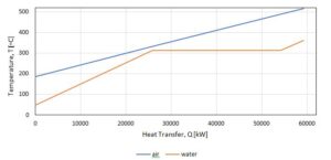
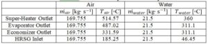
Table 3. HRSG thermodynamic state analysis
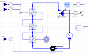
4.4 Combined-cycle power plant model – square in size & broken simulation

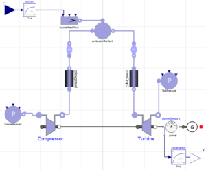
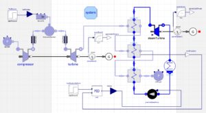
- Figure 9. Combined-cycle power plant model schematic of Diagram view within OMEdit
4.4.1 Combined-cycle power plant assumptions
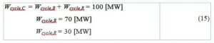
To apply the fundamental continuity equations to our system, there are some model assumptions that need to be made. For the combined-cycle power plant, it is assumed that it is an ideal and reversible cycle. It is also assumed that the fluegas flowing throughout the system will be treated as air, the water flowing throughout the system will be treated as either a liquid, gas, or a two- phase mixture, there will be a minimal 20°C temperature difference between the steam and fluegas, and that the power produced will equal 100 [MW]. The power distribution throughout the system can be exemplified by Equation 15 below.
You can download the Project files here: Download files now. (You must be logged in).
4.4.2 Combined-cycle power plant description
The OpenModelica combined-cycle power plant model consists of one compressor, one combustion chamber, one combustion turbine, one steam turbine, one condenser, one pump, one pressure source, one pressure sink, one mass flow rate regulator, two pressure drops, two generators, three heat exchangers (1 economizer, 1 evaporator, and 1 super-heater), several sources, and several gas state readers. This model consists of one closed loop for the water/steam cycle and one open loop for the fluegas. An important feature of this model is that the thermodynamic cycle is completely closed through the condenser.
5. Modeling Discussion – Informal Narrative
Model building methodology changed quite a bit for myself during my 2019 Spring Science Undergraduate Laboratory Internship (SULI) appointment when I was first introduced to OpenModelica. This can be attributed to who and what I was learning from at the time. With OpenModelica being an open source software package, there is no commercial product support to reach out to when issues arise. This was the main obstacle I faced when learning and modeling in OpenModelica. As a result, I reached out to multiple OpenModelica support forums: openmodelica.org/forum, trac.openmodelica.org, stackoverflow.com, researchgate.com, etc. I found this to be hit or a miss method when troubleshooting issues because responses from site admins happened sporadically and often did not lead to conclusive answers. However, many OpenModelica software developers (Peter Fritzson, Francesco Casella, Adrian Pop, Martin Sjölund, etc.) are active admins on these sites, which is ultimately the best resource anyone could ask for when troubleshooting errors or bugs. What I was learning with, pertains to the OpenModelica literature I was able to find and how relevant the information was to my research. OpenModelica software developers are very active publishers within the OpenModelica science community. The challenge I faced was finding relevant information toward my project and scope of OpenModelica expertise. I remember always feeling as though my modeling experience was in the middle ground between beginner level and advanced level modeling. I seldom found literature material within my intermediate level of modeling and attribute this to the lack of running models I was able to produce during my internship term. During this time of learning to model within OpenModelica, I conducted three phases of model building methodology that progressed as I learned more about the software and techniques associated with building a working model.
5.1 Phase 1 – Brayton and Rankine modeling
Modeling the Brayton and Rankine power cycles on OpenModelica was the first step at being able to model a combined-cycle power plant. Early power cycle models of mine were initially based off the Brayton and Rankine example models found within the MSL. This established a reference point on how I should model these power cycles and what types components I should use from the MSL. In doing so, I gained an understanding of how to parametrize my system’s components, a general idea on how much power should be produced, and general system tendencies. Working with the MSL power cycle example models provided enough hands-on experience to start and replicate my own versions of these models.
Creating my own Brayton and Rankine power cycle models started with satisfying the combined- cycle power plant prescribed power load of 100 [MW]. These two power cycle models need to effectively work together and meet this load. This shared duty can be exemplified in Equations (12), (13), and (15), where the Brayton cycle should produce 70 [MW] and the Rankine cycle should produce an additional 30 [MW]. To compute the inputs needed for the combined-cycle power plant model, inverse computation with respect to the prescribed power load was conducted in order to determine the prescribed mass flow rates for the Brayton and Rankine power cycle models [7]. A thermodynamic state analysis was conducted for both power cycles to produce the required power respectively. System assumptions and the respected state variable values that were solved for can be found in Tables 1 & 2. The thermodynamic state analysis provided the necessary information to act as input parameters for the Brayton, Rankine, and combined-cycle power plant modeling within OpenModelica.
The power cycle models built within OpenModelica can be found in Figures 3 & 6. The Brayton power cycle model was square in size, able to flatten (instantiate), and was able to conduct consistent simulations. A measure of power versus time steady-state simulation plot can be seen in Figure 5. However, although the model was able to be flatten and simulate, there was still a lot of confusion associated with simulation results and general system tendencies. For instance, to change the power output of the Brayton cycle model, mass flow rates were increased and decreased to explore this parameter. The mass flow rate of a system should directly affect the outputs of a power cycle, however power output values stayed constant. Another point of confusion was how the time constant parameter of a simulation works. Often, simulations were executed at the system default of t = 1 second, but upon changing the time constant to a larger more realistic value, the transient simulation would break. Other times, OpenModelica would demonstrate the opposite of this, and would only be able to perform steady-state simulations over extended periods of time and fail upon a simulation at t = 1 second. These system tendencies were a large frustration of mine for I felt the introductory OpenModelica lessons and tutorials did not prepare me for these discrepancies.
The Rankine power cycle model was square in size, unable to flatten (instantiate), and as a result of not being able to flatten, the model failed during simulation. My dysfunctional Rankine power cycle model was a frustration of mine throughout my time using OpenModelica for several reasons. The first frustration of mine pertains to the inconsistent nature of the Rankine example model found within the MSL. Although the Rankine example model was square in size and was able to flatten (instantiate), the model would almost always fail during simulation. The frustrating part for myself was that the model was able to perform successful simulations a handful of random times without warning. The software inconsistencies were a point of confusion I was never able to overcome, which inherently made it difficult to establish a basis of understanding when using OpenModelica.
5.2 Phase 2 – Sub-assembly modeling
Imitating and replicating the Brayton and Rankine example models from the MSL provided a lot of education when building a complex system model, but it only got me so far. Most of my models broke during flattening (instantiation) or would later break during a simulation study. At this point I pivoted in project direction and started to model sub-assemblies of the power cycles. I justified this decision because I was unable to properly troubleshoot the errors associated with my models and did not fully understand each component’s nature and tendencies.
Modeling the sub-assemblies of the larger power cycle models helped establish knowledge for the main components used in the Brayton and Rankine power cycles. Sub-assembly modeling mainly consisted of modeling a single component of interest (i.e. compressor, turbine, heat exchanger, etc.) with other relevant components to facilitate an exchange of information between them. The goal was to simply validate the model’s accuracy and reliability with hand calculations. Keeping sub-assembly models simple was also an important goal of this phase. Flattening and simulating these smaller models was significantly more successful compared to building model systems from scratch. One point of emphasis with this modeling technique is to be skeptical of the simulation results. For a few instances, hand calculations were verified against the simulation results in order to validate a model’s reliability and yielded different results.
You can download the Project files here: Download files now. (You must be logged in).
5.3 Phase 3 – HRSG modeling
Creating sub-assembly models for all the different components used within a combined-cycle power plant model really helped improve my understanding on how each component is used and acts. However, this endeavor never ended up helping me create a working combined-cycle power plant model. Fortunately, right around this time My modeling issues within OpenModelica, Bouskela suggested that I build my model gradually, give realistic values to the boundary conditions and known states via inverse computation, and to start the model building process at a point of fixed pressure.
I decided to try building the combined-cycle power plant model incorporating these ideas by starting at the constant pressure HRSG sub-assembly. Based off my thermodynamic analysis for the Rankine power cycle, I needed to determine the physical characteristics (i.e. material choice, surface area, volume, etc.) of the three heat exchangers that will be used in the HRSG model that will meet the prescribed physical states of the water/steam. A heat exchanger “pinch analysis” was conducted in order to determine heat exchanger characteristics, maximize the HRSG’s efficiency, and to maintain a prescribed 20-degree temperature difference between the fluegas and steam.
The HRSG model seen in Figure 7 was square in size, unable to flatten (instantiate), and as a result of not being able to flatten, the model failed during simulation. The failure of this model indicates that the work completed in this model building process was not enough to produce a model that could flatten, let alone simulate. At this point I had exhausted all my OpenModelica model building strategies for the combined-cycle power plant model. A broken combined-cycle power plant model can be seen in Figure 9.
6. Conclusion
Modelica’s acausal EOO language shows powerful, promising modeling capabilities across multi- domain platforms. The modeling capabilities of OpenModelica were explored through model iterations of the combined-cycle power plant model where only the Brayton power cycle was able to properly work and simulate case studies. The rest of the model iterations did not function properly and broke during simulation due to lack of modeling expertise. Despite most modeling iterations failing during simulation, the thermal energy storage system could be modeled based on this explorative work within OpenModelica due to its ability to act as an opensource and flexible tool for researching renewable energy technologies.
References
- El Hefni, Energy Procedia 49, 1127 (2014).
- Modelica Association, Consortium, Open Source (n.d.).
- Modelica Association, (2013).
- Fritzson, Introduction to Modeling and Simulation with Modelica Using OpenModelica (2012).
- Modelica Association, 1 (2013).
- Scaglioni, YouTube (2013).
- El Hefni, D. Bouskela, B. El Hefni, and D. Bouskela, Modeling and Simulation of Thermal Power Plants (2019).
- Press, G.W. Arnold, P. Mak, and R. Perez, Principles of Object Oriented Modeling and Simulation (n.d.).
- Sjölund, Tools and Methods for Analysis, Debugging, and Performance Improvement of Equation-Based Models (2015).
- Wendelin, A. Dobos, A. Lewandowski, T. Wendelin, and A. Dobos, (2013).
- Fritzson and P. Bunus, Proc. – Simul. Symp. 2002–January, 365 (2002).
You can download the Project files here: Download files now. (You must be logged in).
Keywords: Thermodynamic, Combined-Cycle, Power Plants, Open Modelica


Responses