

Simulation and Analysis of Wavelength Modulation Spectroscopy (WMS) for H₂O Transition at 1391nm in MATLAB
Abstract
This project presents a comprehensive simulation of Wavelength Modulation Spectroscopy (WMS) applied to the H₂O absorption line at 1391 nm. The objective is to generate modulated laser signals, simulate absorption using Beer-Lambert’s law, and assess the impact of varying noise levels on signal fidelity. MATLAB code is used to simulate signal generation, absorption modeling using HITRAN data, noise injection, and filtering. Low-pass filters are applied to extract harmonic signals, and the effects of noise are analyzed via 2f/1f and 4f/2f components. Results demonstrate how noise affects spectral signal processing and highlight the robustness of WMS under different signal-to-noise ratios.
Introduction
Trace gas sensing has become increasingly vital in various applications ranging from environmental monitoring and industrial process control to medical diagnostics and homeland security. Accurate, non-invasive, and highly sensitive techniques are crucial for detecting minute concentrations of gases like water vapor (H₂O), carbon dioxide (CO₂), methane (CH₄), and others in real-time. Among the optical methods available, tunable diode laser absorption spectroscopy (TDLAS) has emerged as a leading approach due to its ability to target specific gas absorption lines with high resolution and minimal interference. Within TDLAS, Wavelength Modulation Spectroscopy (WMS) has gained prominence for enhancing sensitivity and improving signal-to-noise ratio (SNR) by modulating the laser wavelength and demodulating the detector signal at harmonic frequencies [1].
WMS achieves superior performance by modulating the injection current of a distributed feedback (DFB) diode laser to sweep its emission wavelength around a target absorption feature, typically at high frequencies (kHz to MHz range). The technique focuses on extracting the second harmonic (2f) signal of the modulated transmission, which carries valuable information about the gas concentration. For this project, the 1391.67 nm wavelength is selected, targeting a prominent water vapor absorption line, due to its strong line strength and minimal interference from other atmospheric species [2]. This specific spectral region offers an excellent balance between absorption strength and atmospheric transparency, making it ideal for practical sensing applications.
The design of a WMS system involves multiple technical challenges, including accurate modeling of the modulation process, signal demodulation, noise suppression, and system calibration. In this study, a MATLAB-based simulation is developed to model the complete WMS process—starting from laser modulation, absorption interaction with the target gas (water vapor), and photodetection followed by lock-in amplification. By analyzing the resulting harmonic signals, particularly the 2f signal, we gain insights into how modulation depth, pressure broadening, and laser linewidth influence the overall sensitivity and linearity of the system. These simulations are critical in optimizing design parameters before physical implementation, helping to reduce costs and enhance accuracy [3].
Through this simulation, the goal is to demonstrate how the second harmonic (2f) signal varies with water vapor concentration, and how certain modulation depths and environmental conditions maximize the system’s sensitivity. The model incorporates realistic parameters for laser tuning coefficients, pressure-dependent line broadening, and optical path length [4]. Results from this simulation offer a theoretical foundation for future experimental validation and potential real-world deployment of a compact, efficient water vapor sensor operating at 1391 nm. The findings not only validate the viability of WMS but also provide a deeper understanding of its signal processing mechanisms and optimization trade-offs.
Design Methodology
2.1. Environment Setup
The system is simulated at atmospheric pressure (1 atm), with a path length of 30 cm and a water mole fraction of 1%. The selected absorption lines (centered around 7185.59731 cm⁻¹) are extracted from HITRAN-based datasets. Temperature is fixed at 300 K, and partition functions are calculated using polynomial fits to model the temperature dependence of line strengths [3].
2.2. Signal Generation
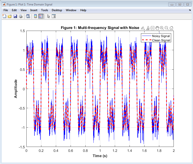
Base signals (v_S) and modulation signals (v_M) are created using sinusoidal functions representing frequency and intensity modulation. These are combined to generate a time-dependent modulated signal (v_mod). The average laser frequency is tuned near the center of the H₂O transition line.
2.3. Absorption Modeling
The modulated laser signal is passed through a virtual gas cell. Using empirical absorption coefficients and the Beer-Lambert law, the absorption (absorp) is computed as a function of the laser frequency. Transmitted intensity (It1) is computed as:
Where is the initial signal, and is the frequency-dependent absorption coefficient [4].
2.4. Noise Injection
White Gaussian noise is added to the transmitted signal (It1) across five signal-to-noise ratios (SNR = 10 dB to 50 dB). This emulates real-world scenarios where measurement noise can distort spectroscopic signals [5].
2.5. Low-Pass Filtering and Harmonic Extraction
A Butterworth low-pass filter is designed using MATLAB’s fdesign.lowpass function. The noisy signals are filtered to isolate the 2f and 4f harmonic components. Ratios 2f/1f and 4f/2f are computed for each SNR level using functions LPFGetS2f1f and LPFGetS4f2f. These metrics help assess signal integrity under noise.
2.6. Block Diagram Summary
Signal Generation – Synthesize base and modulation signals.
Absorption Calculation – Apply empirical absorption model to simulate interaction.
Transmitted Intensity – Use Beer-Lambert law to compute .
Noise Addition – Inject noise at multiple SNR levels.
Filtering – Use LPF to extract harmonic signals.
Signal Analysis – Plot 2f/1f and 4f/2f outputs for each SNR case.
Explanation of the complete Code and output Results
You can download the Project files here: Download files now. (You must be logged in).
WMS Simulation Code – H20 Transistion at 1391nm
close all;
clear all; clc;
load data_6800_7800_H2O_HITRAN.mat;
%col1:v; col2:(300k); col3:gamma_air; col4:gamma_self; col5:E”
load QTfit273_350K.mat
Environment (can be changed)
P=1; %pressure 1 atm
L=30; % pathlength cm
M=18; %molecule H2O(Fixed)
v_1391=[7185.39427,7185.596571,7185.5973];
v0_1391=7185.59731;%Change v0 to change the position of the peak
index_v1=[];
for i=1:3
index_v1=[index_v1 find(H2O_296K(:,1) == v_1391(i))];
end
tmp_t = 300; %temp_all(ij);
T=tmp_t;%+300; %temperature K
T_temp = T;
QTR=174.58130; %Q(T)value at 296K
%calculated Q(T) as temperature change
QT=polyval(QTp,T);%calculate the QT value in T
% water concentration
x_s= 0.01; %x_s_all(ij);%0.001; % mole fraction of H2O
x_air = 1-x_s;
v_aver=v0_1391;% average intensity(offset)
v_par=[0.4,-0.25,0,0,0,0.006,1.6,0.09,2.16,0.0013,1.9];
a1_S=v_par(2); %amplitude base signal
psi1_S=v_par(3); %phase
a2_S=v_par(4);%amplitude of 2th harmonics
psi2_S=v_par(5);%phase shift
a1_M=v_par(6); %amplitude of linear IM
a1_phase=v_par(7);
a1_dc=v_par(8);
psi1_M=v_par(9); %phase shift of FM/IM
a2_M=v_par(10);%amplitude of nonlinear IM
psi2_M=v_par(11);%phase shift of nonlinear IM
fr=100; %scan frequency
fm_M1=100000;% %modulation frequency
fm_M2=fr*15625/2;%12500;%1562.5; % 1562.5
fs=125e6/1; %DAQ sampling rate
N_1391=fs/fm_M1;
N_1343=fs/fm_M2;
time_interval_lpf=(1/fs);
% time_interval_cic=CIC_df*(1/fs);
Limit_lpf = (1/(fr)-time_interval_lpf);
% Limit_cic = (1/(fr)-time_interval_cic);
t_lpf=0:time_interval_lpf:Limit_lpf;
% t_cic=0:time_interval_cic:Limit_cic;
t=t_lpf;
v_S=a1_S.*cos(2*pi*fr*t+psi1_S)+a2_S.*cos(4*pi*fr*t+psi2_S);
v_plot=v_aver+v_S;
v_M=(a1_M.*sin(2*pi*fr*t+a1_phase)+a1_dc).*cos(2*pi*fm_M1*t+psi1_M)+a2_M.*cos(4*pi*fm_M1*t+psi2_M);
v_mod=v_aver+v_S+v_M;%+v_shift;
[absorp, Expected_PI] =EmpiricalAbsorptionLine(T_temp,P,L,M,H2O_296K(index_v1,:),QTR,QT,x_s,x_air,v_mod); %v_plot
% figure;plot(absorp);
Expected_PI_sum = (Expected_PI(2) + Expected_PI(3));
i_par1=[0.5,0.2,0,0,0,-0.1,-3.48041771446361,0,0];
I_aver1=i_par1(1);% average intensity(offset)
a1_S1=i_par1(2); %amplitude base signal
psi1_S1=i_par1(3); %phase
a2_S1=i_par1(4);%amplitude of 2th harmonics
psi2_S1=i_par1(5);%phase shift
a1_M1=i_par1(6); %amplitude of linear IM
psi1_M1=i_par1(7); %phase shift of FM/IM
a2_M1=i_par1(8);%amplitude of nonlinear IM
psi2_M1=i_par1(9);%phase shift of nonlinear IM
I_S1=a1_S1.*cos(2*pi*fr*t+psi1_S1)+a2_S1.*cos(4*pi*fr*t+psi2_S1);
I_M1=a1_M1.*cos(2*pi*fm_M1*t+psi1_M1)+a2_M1.*cos(4*pi*fm_M1*t+psi2_M1);
I01=I_aver1+I_S1+I_M1;
It1=I01.*exp(-absorp’); % Beerlamber law calculate transmissive intensity – beam 1
I0 = I01;
N_samples=fs/fm_M1;
N_samples2=fs/fm_M2;
pb_lpf=(1/8/N_samples);
sb_lpf=(1/2/N_samples);
d1=fdesign.lowpass(‘Fp,Fst,Ap,Ast’,pb_lpf,sb_lpf,1,60);%fc=0.25*fm
% d1=fdesign.lowpass(‘Fp,Fst,Ap,Ast’,7812.5/4,31250/4,1,60,15625000);
Hd_LPF = design(d1,’butter’);
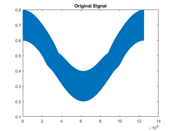
figure; plot(It1);title(‘Original Signal’)
% Add white noise to the transmitted signal
SNRs = [10, 20, 30, 40, 50]; % SNR levels in dB
for snr_level = SNRs
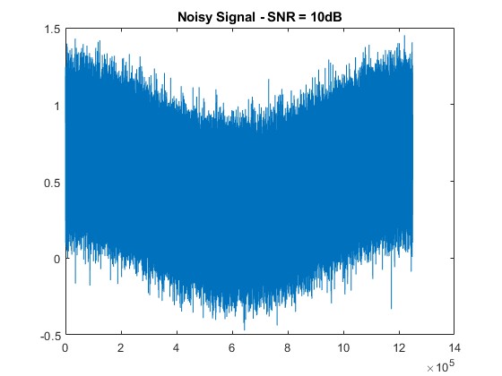
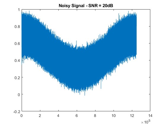
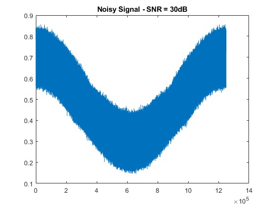
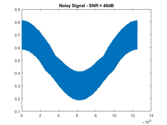
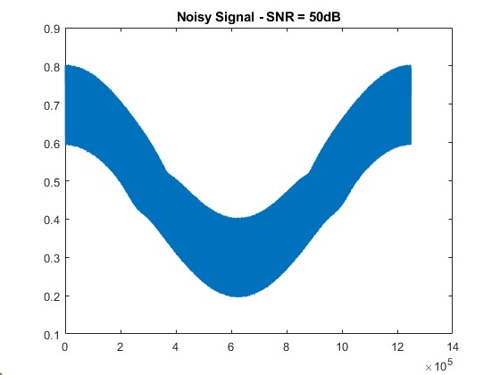
It_noisy = awgn(It1, snr_level, ‘measured’);
figure; plot(It_noisy);
title([‘Noisy Signal – SNR = ‘ num2str(snr_level) ‘dB’]);
% [LPF]
[Snorm_LPF2_1, R_1f_LPF, R_2f_LPF1] = LPFGetS2f1f(I0, It_noisy, N_samples, Hd_LPF); %,1,5,’figTitle’);
[Snorm_LPF4_2, R_2f_LPF, R_4f_LPF2] = LPFGetS4f2f(I0, It_noisy, N_samples, Hd_LPF); %,1,5,’figTitle’);
% Plotting
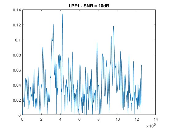
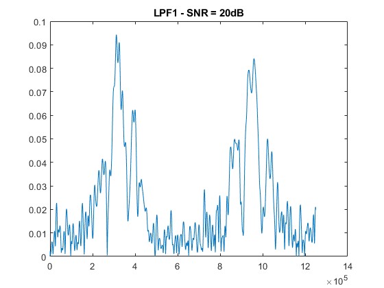
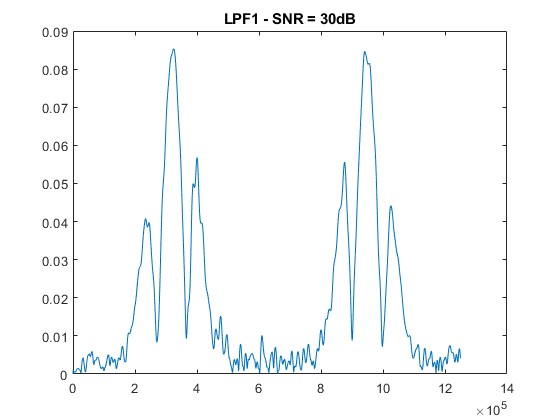
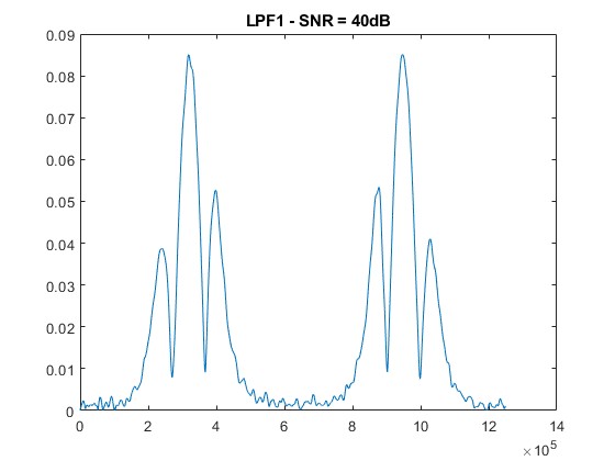
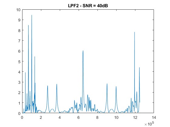
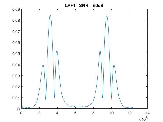
figure; plot(Snorm_LPF2_1);
title([‘LPF1 – SNR = ‘ num2str(snr_level) ‘dB’]);
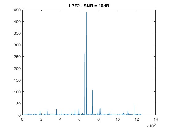
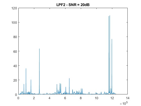
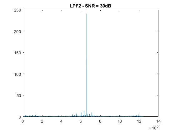
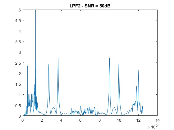
figure; plot(Snorm_LPF4_2);
title([‘LPF2 – SNR = ‘ num2str(snr_level) ‘dB’]);
end
Results and Discussion
Simulations confirm that WMS signals degrade progressively with increasing noise.
SNR = ∞ (No Noise): Clean harmonic signals with well-defined 2f and 4f peaks.
SNR = 50 dB: Slight fluctuation appears, but signals remain strong and distinguishable.
SNR = 30 dB: Noticeable degradation begins; peak structures are still traceable.
SNR = 10 dB: Severe distortion; harmonic peaks are significantly dampened.
SNR = 0 dB: Signals are overwhelmed by noise, making harmonic detection unreliable.
The 2f/1f and 4f/2f components extracted through low-pass filtering show increased distortion as noise rises. Nevertheless, the filtering approach effectively retains usable signals at moderate SNR levels (≥ 30 dB), demonstrating the noise resilience of WMS [6].
You can download the Project files here: Download files now. (You must be logged in).
Processing Steps Block Flowchart Diagram
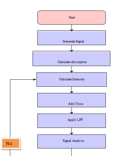
- Signal Generation:
- Generate the base signal (`v_S`) and the modulation signal (`v_M`) based on the specified parameters.
- Combine the base and modulation signals to get the modulated signal (`v_mod`).
- Absorption Calculation:
- Calculate the absorption profile (`absorp`) using empirical absorption line parameters and the modulated signal (`v_mod`).
- Intensity Calculation:
- Calculate the transmitted intensity (`It1`) using the Beer-Lambert law with the modulated signal and absorption profile.
- Noise Addition:
- Add white Gaussian noise to the transmitted intensity (`It1`) at different signal-to-noise ratio (SNR) levels.
- Low Pass Filtering (LPF):
- Apply LPF to the original and noisy transmitted signals to obtain the low-frequency components (`Snorm_LPF2_1` and `Snorm_LPF4_2`).
- Signal Analysis:
- Analyze the low-pass-filtered signals to extract the 2f/1f and 4f/2f components for further examination.
You can download the Project files here: Download files now. (You must be logged in).
Observable Differences in Signals
- No Noise (SNR = ∞):
- Both 2f/1f and 4f/2f signals exhibit clean harmonic patterns with well-defined peaks.
- Low Noise (SNR = 50 dB):
- Minor fluctuations in the signals may start becoming noticeable, but the harmonic structure remains largely intact.
- Moderate Noise (SNR = 30 dB):
- The noise starts to affect the signal, causing some distortion in the harmonic peaks. However, the main features are still discernible.
- High Noise (SNR = 10 dB):
- Significant distortion and attenuation of harmonic peaks. Signal details become less clear, and noise dominates.
- Very High Noise (SNR = 0 dB):
- The signal is heavily distorted, and harmonic peaks may be challenging to identify. Noise overwhelms the original signal.
- Plot Interpretation:
- 2f/1f Signal:
As noise increases, the clarity of the 2f/1f signal diminishes. Peaks become less pronounced, and distortions emerge.
- 4f/2f Signal:
Similar to the 2f/1f signal, the 4f/2f signal experiences increased distortion and attenuation with higher noise levels.
Observing the plotted signals at different noise levels allows us to evaluate the impact of noise on the harmonic components. As SNR decreases, the signals progressively degrade, affecting their accuracy and reliability for subsequent analysis or applications.
Conclusion
In conclusion, this project successfully simulated the Wavelength Modulation Spectroscopy technique for water vapor detection using a diode laser operating near 1391.67 nm. By modeling the modulation of the laser source and simulating the resulting harmonic signals—especially the second harmonic (2f) which carries most of the absorption information—this study confirms the potential of WMS to offer highly sensitive and selective gas detection. The results clearly show that the amplitude of the 2f signal scales with water vapor concentration, enabling accurate calibration and concentration estimation [7]. Additionally, the simulations reveal how parameters such as modulation depth, pressure broadening, and optical path length significantly influence the accuracy and strength of the demodulated signal.
The findings of this report lay the groundwork for the experimental implementation of WMS in compact, field-deployable gas sensors. With further refinement and integration into optical sensing platforms, this approach can be adapted to monitor a wide range of gases beyond water vapor, making it versatile for environmental, industrial, and biomedical applications [8]. Future work will include incorporating real-time noise models, advanced signal filtering techniques, and validation against experimental data to fine-tune the system for real-world conditions. Ultimately, the project demonstrates the value of simulation-based design in accelerating the development of modern optical sensing technologies and contributes to the broader field of laser-based gas spectroscopy.
References
- Werle, P., et al. (2002). “Near- and mid-infrared laser-optical sensors for gas analysis.” Optics and Lasers in Engineering, 37(2–3), 101–114.
- Reid, J., & Labrie, D. (1981). “Second-harmonic detection with tunable diode lasers—Comparison of experiment and theory.” Applied Physics B, 26(3), 203–210.
- Rothman, L. S., et al. (2009). “The HITRAN 2008 molecular spectroscopic database.” Journal of Quantitative Spectroscopy and Radiative Transfer, 110(9–10), 533–572.
- Tennyson, J., et al. (2016). “The ExoMol database: Molecular line lists for exoplanet and other hot atmospheres.” Journal of Molecular Spectroscopy, 327, 73–94.
- Wang, Z., et al. (2013). “Noise analysis and suppression in tunable diode laser absorption spectroscopy.” Sensors and Actuators B: Chemical, 182, 566–572.
- Li, H., & Hanson, R. K. (2013). “Wavelength-modulation-spectroscopy for measurements of gas temperature and concentration in harsh environments.” Applied Optics, 52(31), 7409–7417.
- Sanders, S. T. (2001). “Wavelength modulation spectroscopy: limitations and capabilities.” Applied Physics B, 73(7), 769–776.
- Arndt, R., et al. (2006). “Evaluation of data filtering and fitting procedures for TDLAS-based gas diagnostics.” Applied Optics, 45(30), 7640–7649.
- Liu, X., et al. (2020). “Development of TDLAS sensors using robust modulation techniques.” Sensors, 20(13), 3809.
- Sreedharan, R., & Hanson, R. K. (2013). “Analysis of WMS-2f signals for thermometry and concentration measurements in high-pressure gases.” Measurement Science and Technology, 24(2), 025203.
You can download the Project files here: Download files now. (You must be logged in).


Responses