

Virtual sensing for SHM: a comparison between Kalman filters and Gaussian Processes
Author: Waqas Javaid
Abstract
Structural Health Monitoring (SHM), is a very active research field, aimed at producing methodologies for the periodic, and often online, assessment of structures. While there are different approaches, and perhaps definitions for SHM, there is one common necessary element if applied in practice: data acquired from sensors. In an ideal scenario, sensors could be deployed anywhere on a structure of interest, and could be added retrospectively, if not included in the original design. In practice, there are limitations to the availability and installation of sensors, such as physical access and cost. Virtual sensing has thus been proposed as a solution to the problem of sensor availability and different approaches have been applied in various fields. This paper explores and compares two approaches for virtual sensing in structural dynamics: Kalman filters and Gaussian process regression – with the ultimate purpose of assessing their suitability for SHM. The approaches are demonstrated on data from a laboratory structure: a nonlinear Brake-Reuß beam.
1 Introduction
Monitoring the state of structures is vital for their continued safe operation, and also for the efficient man- agement of their maintenance. Structural Health Monitoring (SHM), refers essentially to any process that involves a periodic or on-line assessment of a structure, and is a very active research field; comprehensive reviews can be found in [1, 2]. While there are many different approaches to SHM, there is one common necessary element if applied in practice – data acquired from sensors. Without reliable sensors to provide data, no SHM approach can work, regardless of whether it is physics-based or data-driven. In an ideal sce- nario, sensors could be installed anywhere on a structure of interest and could be added retrospectively if required. In practice this is not usually possible as there are limitations in terms of cost and physical ac- cess. Retrospective fitting can be expensive or practically unfeasible, while inclusion in the original design is costly or perhaps impossible without a priori knowledge. Virtual sensing has been proposed as a solution to the problem of sensor availability and is also an active research area.
In fact, virtual sensing has been of interest in various fields and may be reported under different terminologies in the literature. Some examples include: control applications [3] and active noise control [4], monitoring of nuclear power facilities [5], diesel engine emissions [6], on-chip temperature estimation [7], even in crowd dynamics [8]. Various approaches to virtual sensing have been tried; among them, Kalman filters are a popular choice [9, 10], Extended Kalman Filters [11] including their combination with neural networks have also been used [12], h-infinity virtual sensors [13] and also machine learning algorithms such as Gaussian Processes (GPs) [5, 14, 15], or Gaussian Mixture Regression [16].
In structural dynamics virtual sensing has made use of Kalman filters [10, 17], dynamic sub structuring [18, 19] and modal expansion [20, 21]. The latter includes applications in wind turbines [22] and has been compared with Kalman filters [23]. Usually in structural dynamics, the aim is to either infer measurements into unknown (unmeasured) locations and/or to estimate full-field deformation (and strain) of the entire structure of interest. Although GP regression has been used in some form for virtual sensing in other fields, it has not been applied widely in structural dynamics. The purpose of this paper is to explore, compare and demonstrate two approaches: Kalman filtering and GP regression. The work is demonstrated with the help of a nonlinear Brake-Reuß beam [24] which is tested under laboratory conditions.
The layout of this paper is as follows: the next section presents the mathematical formulation for the two approaches which are used for virtual sensing. The third section describes the structure and experimental setup as well as the FE modelling of the structure. Section four presents the results and compares the two approaches. Finally, a short conclusion recaps the work in order to round off the paper.
2 Problem formulation
The problem of virtual sensing pertains to the inference of the dynamic response at unmeasured system loca- tions, the so-called virtual sensing points, on the basis of sparse vibration measurements. Within this context, the process of virtual sensing consists in extrapolating the measured vibration response by means of informa- tive model structures, which are able to accurately estimate the engineering quantities of interest at the virtual sensing locations. Depending on the type of extrapolator, virtual sensing can be classified into physics-based or data-driven techniques, such as Modal Expansion or Gaussian-Process regression respectively, while an additional classification exists between deterministic and stochastic approaches, such as Modal Expansion and Bayesian filtering, respectively. This section presents the mathematical formulation of the two stochastic techniques that will be considered in this paper; namely, Bayesian filtering and Gaussian Process regression, which are further categorised as physics-based and data-driven respectively.
You can download the Project files here: Download files now. (You must be logged in).
2.1 Bayesian filtering
In the context of Bayesian-based virtual sensing, the underlying system dynamics are typically represented by a physics-based model, which is expressed in a stochastic discrete-time state-space form:
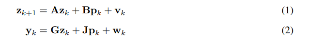
where zk and yk are the state and output vectors, pk is the input vector, A and B are the system matrices, G and J are the output and direct transmission matrices, while vk and wk represent the process and measurement noise terms, respectively. The state equation matrices depend on the system mass, damping and stiffness matrices M, C and K respectively, while the structure of the measurement equation matrices depends on the observed response quantities.
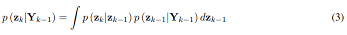
The problem of sequential Bayesian inference, which is oftentimes referred to as Bayesian filtering, consists in recursively estimating the prior probability density function p (zk|Yk−1), at time k, given the posterior p (zk−1|Yk−1) at time k − 1 and subsequently the posterior probability density function p (zk|Yk), which implies availability of measurements up to and including time k. The calculation of the prior density is based on the process model, described by Eq. (1):
As well as on the Markovian property, which postulates that p (zk|zk−1, Yk−1) = p (zk|Yk−1). The posterior step can be carried out using Bayes’ theorem,
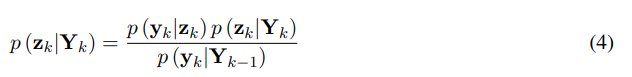
This can be rewritten in a recursive formula:

Where the likelihood p (yk|zk) is defined from the measurement equation of the state-space representation. The estimation of the posterior probability density function enables the extraction of the state statistical moments, with the first two being usually of interest in typical engineering applications:
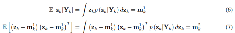
with E[·] denoting the expectation operator. In the particular case of Linear Time Invariant (LTI) systems with additive Gaussian noise, as postulated by Eqs. (1) and (2), the solution of Eqs. (6) and (7) is obtained by the well known Kalman filter. The implementation of a Kalman filter for virtual sensing requires availability of
the input signals that drive the system dynamics. In the absence of such information, the response estimates can be obtained by means of an output-only filtering approach, such as the Augmented Kalman Filter (AKF), the Dual Kalman Filter (DKF) or the Joint input-state estimator by Gillijns and De Moor [25].
2.2 Gaussian Process regression
Rasmussen and Williams [26] define a Gaussian process (GP) as “a collection of random variables, any finite number of which have a joint Gaussian distribution”. A GP is thus completely defined by a mean m(x) and a covariance function k(x, x′), where x represents the input vector. So for any real process f (x) one can define,
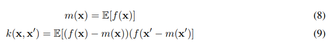
Where E represents the expectation. Often, for practical reasons because of notation purposes (simplicity) and little knowledge about the data at the initial stage, the prior mean function is set to zero. The Gaussian processes can be defined as,
![]()
If a zero-mean function is assumed, the covariance function can be described as,

this is the squared-exponential covariance function which is used throughout this paper, for other choices of covariance functions the reader is referred to [26]. Assuming now that one has a set of training outputs f , and a set of test outputs f ∗, one has the prior [26],
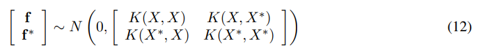
Where the capital letters represent matrices. If there are n training points, and n∗ testing points, then K(X, X∗) denotes the n × n∗ matrix of the covariances evaluated at all pairs of training and test points, and similarly for the rest of the matrices K(X, X), K(X∗, X) and K(X∗, X∗).
As the prior has been generated by the mean and covariance functions, in order to specify the posterior distribution over the functions, one needs to limit the prior distribution in a such a way that includes only these functions that agree with actual data points. In a probabilistic manner this can be done easily via conditioning the joint prior on the observations and this will give (for more details see [26],
![]()
Function values f ∗ can be generated by sampling from the joint posterior distribution and at the same time evaluating the mean and covariance matrices from (13).
In practice, it may not be possible to access function values themselves, but rather noisy versions: y = f (x) + ϵ. Assuming i.i.d. Gaussian noise ϵ with variance σ2, then equation (13) becomes [Rasmussen],

Covariance functions are typically accompanied by some extra parameters in order to obtain a better control over the types of functions that are considered for the inference. The squared-exponential covariance function can take the form (1 dimensional),

Where ky is the covariance for the noisy target set y. The length-scale l (determines how far one needs to move in input space for the function values to become uncorrelated), the variance σ2 of the signal, and the noisy variance σ2 are free parameters that can be varied. These free parameters are called hyperparameters.
Optimal hyperparameters for GP regression, can be chosen with the help of the maximum marginal likelihood of the predictions p(y|X, θ) with respect to the hyperparameters θ,
![]()
where Ky = Kf + σ2I is the covariance matrix of the noisy test set y and Kf is the noise-free covariance matrix. The reader is referred again to [26] for the exact solution of the maximisation of the marginal log likelihood through its partial derivatives.
For the purposes of virtual sensing, GP regression is used here when x consists of the time data of 1 or more sensors, and the target data y is the time response of a sensor of interest. The software used for the implementation of GP regression was provided by [26].
2.3 Performance assessment
When comparing time traces, it may be typical to use the Time Response Assurance Criterion (TRAC) [20]. Similar to the Modal Assurance Criterion (MAC) [27], TRAC is defined by,
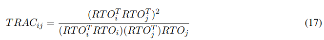
where RTOi and RTOj represent the time signals at points i and j. TRAC takes values between 0 and 1 – here it will also be presented in percentage.
The TRAC does not take into account scaling, so in order to check the quality of estimates, the normalised mean-square error (MSE) is also used,
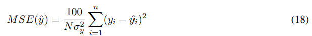
where the caret denotes an estimated quantity, yi is the actual observation, N the total number of observations and σy the standard deviation. In general, an MSE error below 5 is considered a good fit and below 1 excellent.
3 Modelling and experimental setup
3.1 Structure and experimental setup
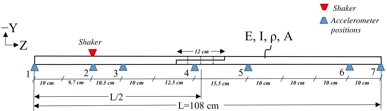
The structure of interest is a Brake-Reuß beam [24], which is composed of two overlapping and identical beams connected through a lap joint interface. Due to the presence of the joint, the structure will exhibit nonlinear response when strongly excited and its modelling may present challenges. The lap joint is secured with three M8 bolts, nuts, and washers at a torque of 20 Nm. In fact, by changing and controlling the torque in the bolts one could introduce a form of ‘damage’ (or pseudo-fault – see [28, 29]) into the structure.
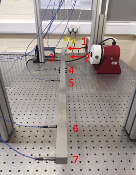
The experimental setup can be seen in Figure 1. The beam was suspended through nylon fishing line to approximate ‘free-free’ boundary conditions and was excited with the help of a Data Physics electromagnetic shaker; its response was recorded through 7 uniaxial accelerometers of the PCB type, attached directly on the structure (see Figures 1 & 2). The excitation force was random and was recorded through a force transducer. The DAQ system consisted of two National Instruments (NI) 9234 modules with a total of 8 channels. In total, 20 sec of time data were recorded with a sampling rate of 25.6 KHz. The data were later filtered through a low-pass Butterworth filter with a cut-off frequency of 550 Hz. Frequency Response Functions (FRFs) were able to be estimated through the time data, although they are not used in this work.
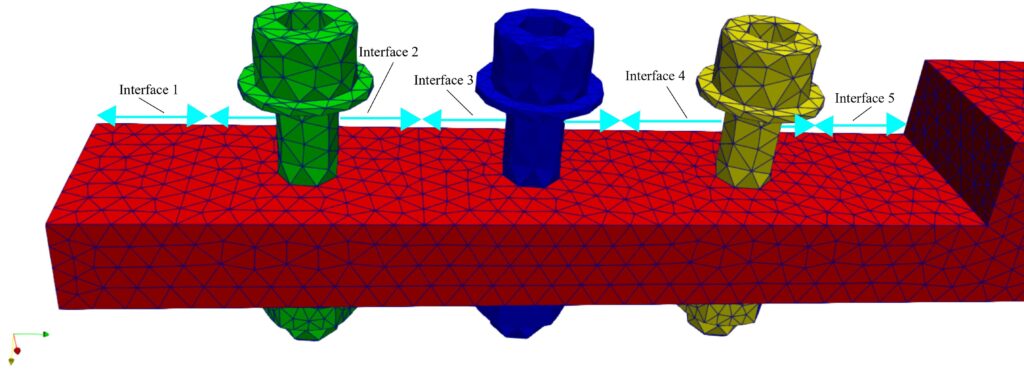
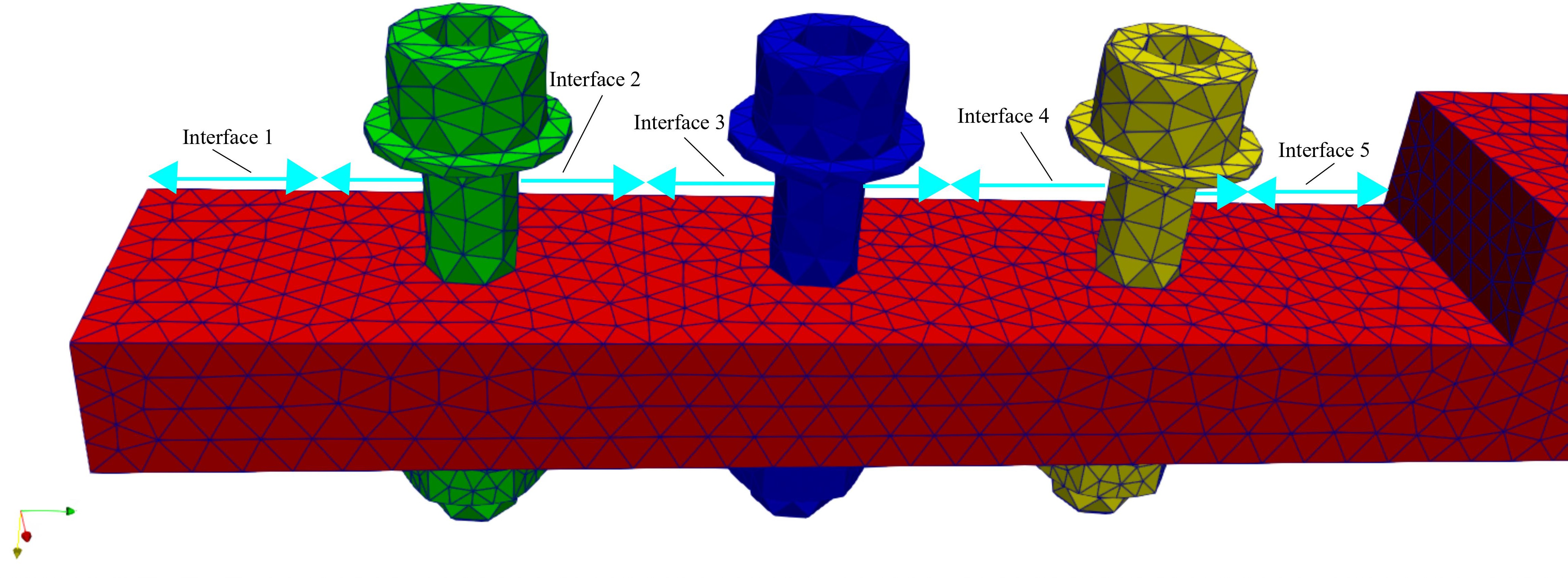 (b) Subdivision of the contact surface between the two beams.
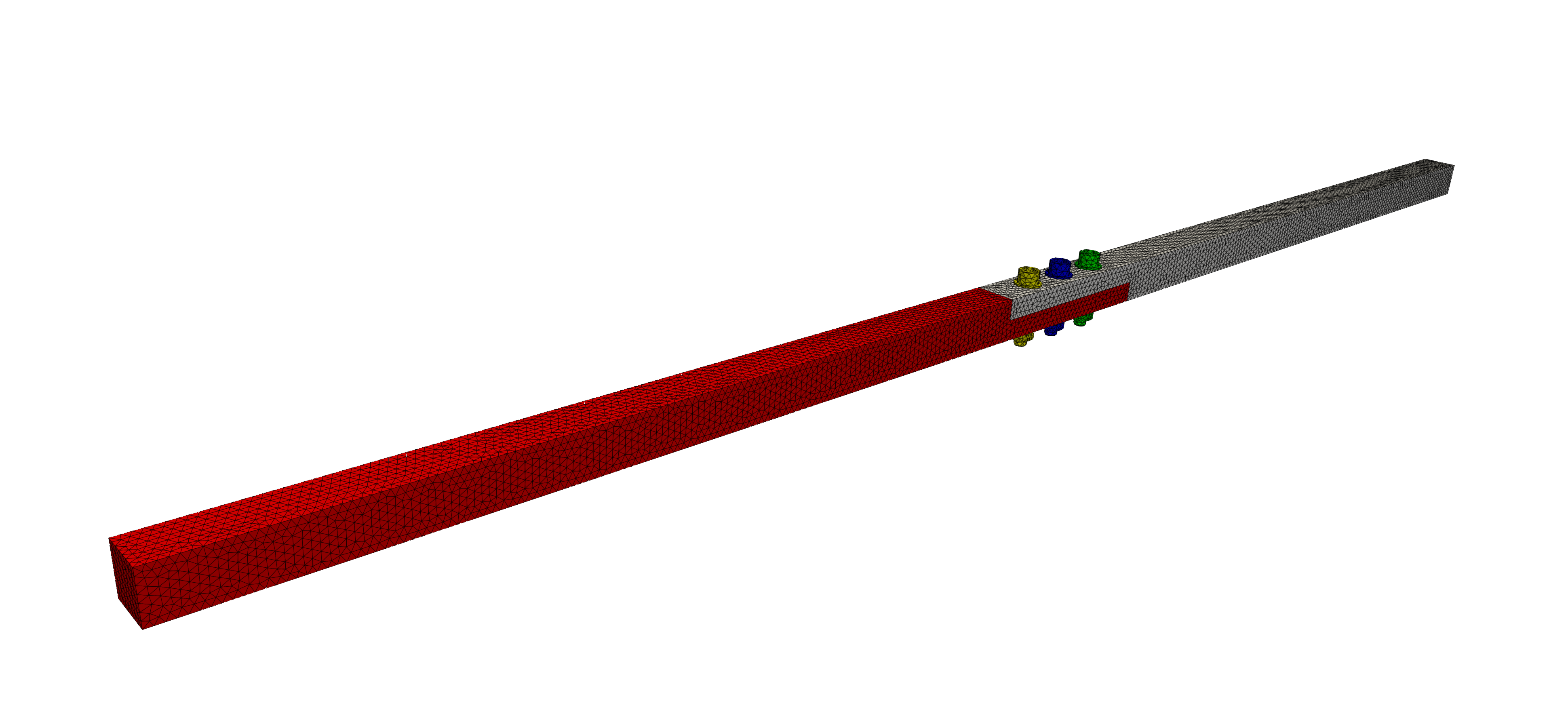
Figure 3: FE modelling of the experimental beam.
You can download the Project files here: Download files now. (You must be logged in).
3.2 Modelling
The beam along with the bolts, nuts and washers were modelled using linear tetrahedral solid elements, as shown in Figure 3a, while interface elements were added in all contact surfaces. The contact surface between the beams, was divided into 5 subsections, as illustrated in Figure 3b, with a different interface element stiffness being used for each section. For the material parameters, nominal values for steel were used.
In order to reduce discrepancies between the model and experimental measurements, the initial model was updated using the sensitivity method [30]. In particular, the stiffness of the beams, bolts and interface ele- ments were updated by minimising the undamped eigenvalue residual. The method of Zhang et al. [31] was employed to impose upper and lower bounds on the updated parameters, thus avoiding physically meaning- less values. Since only accelerations in one direction were measured, modes with zero components along this direction were excluded from the updating process. In Table 1, the predicted natural frequencies before and after updating are compared to the measured ones. It can be seen that the initial predictions are overall improved by updating, achieving a very good agreement with the experimental results.
Table 1: Comparison of predicted and measured natural frequencies before and after updating.
| Mode | Test (Hz) | Initial model (Hz) | Error (%) | Updated model (Hz) | Error (%) |
| 1 | 80.99 | 82.85 | 2.28 | 81.25 | 0.32 |
| 2 | 281.28 | 293.04 | 4.18 | 284.44 | 1.12 |
| 3 | 508.27 | 516.89 | 1.69 | 504.28 | 0.79 |
| 4 | 831.92 | 865.27 | 4.01 | 839.86 | 0.95 |
| 5 | 1307.11 | 1316.81 | 0.74 | 1285.58 | 1.64 |
4 Results
4.1 Bayesian filtering
The Bayesian-based estimates are obtained by combining the numerical model of the system with the avail- able measurements, in order to extrapolate the response at locations where measurements have not been included in the update step. As such, the prediction does not require any training phase and can be per- formed simply by tuning the covariance matrices of the noise terms. It should be noted that the quality of estimates is strongly dependent on the agreement between the numerical model and the system where data were generated from, as well as on the tuning parameters. The results for four different sensor configurations and prediction points are presented in Table 2 in terms of the average MSE and TRAC values, which are obtained from 20 samples of the noise covariance terms (i.e. 20 sets of tuning parameters).
Table 2: Bayesian-based prediction results at unmeasured locations
| Input sensors | Predicted sensor | Mean MSE | Mean TRAC |
| 1,2,4 | 3 | 3.93 | 0.956 |
| 3,4,5 | 2 | 4.15 | 0.926 |
| 4,5,6 | 7 | 2.58 | 0.993 |
| 5,6,7 | 4 | 0.43 | 0.995 |
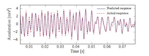
Fig. 4 shows an example of the prediction of sensor 3 by using acceleration data from sensors 1, 2 and 4. The MSE is equal to 6.14 due to the small amplitude discrepancy between the two signals however, the high correlation between the two signals is evidence from the TRAC, which is equal to 96.2%. It should be underlined that the prediction is not based on a training phase and as such, all estimates are obtained on the basis of unseen data.
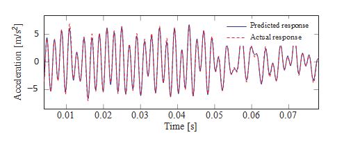
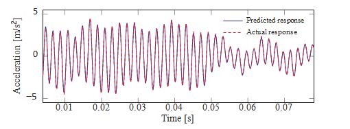
The time series presented in Figs. 5 and 6 correspond to the estimates at sensors 7 and 4 respectively, where a very accurate estimate is obtained in both cases, which are characterized by MSEs smaller than 1 and TRAC values close to 1.
4.2 Gaussian Processes
When using GPs for virtual sensing, the approach made use of the data from some sensors to predict (through regression) the response of another sensor. It was found that at least three sensors were required to predict one, and not all sensors were able to be predicted in a satisfactory way. Due to the large number of training samples the data was randomly separated into training and validation sets (with a 70-30 ratio) and subse- quently randomly sub-sampled.
The final training data had a size of 1200 data points per sensor while for the validation and the calculation of the MSE 10000 samples were used. The random sub-sampling caused variations in the results, so for each configuration (combination of sensors as inputs and output) the training was run 50 times. The overall results can be seen in Table 3 for the prediction of sensors 2,3,4 and 7 through combinations of other sensors. Sensors 1 and 6 were the most challenging to predict through different combinations and had average MSE values of more than 10 after 50 runs, indicating bad regression fits.
Table 3: GP regression sensor prediction results after 50 runs for different configurations. Random sub- sampling created different testing and validation sets for each run.
| Input sensors | Predicted sensor | Mean MSE | best MSE | Mean TRAC % | best TRAC % |
| 1,2,4 | 3 | 4.5 | 0.84 | 96 | 99 |
| 3,4,5 | 2 | 5.67 | 1.83 | 95 | 98 |
| 4,5,6 | 7 | 5.11 | 0.59 | 96 | 99 |
| 5,6,7 | 4 | 6.69 | 1.26 | 94 | 99 |
Figure 7 shows an example of the prediction of sensor 3 by using acceleration data from sensors 1,2 and 4. It is noted here that since this is treated as a regression problem, the input/target sets are normalised between
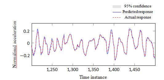
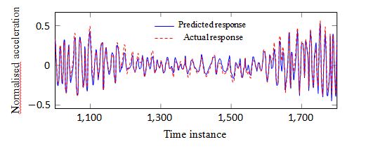
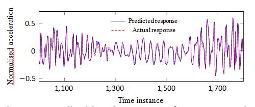
-1 and 1. The MSE of 1.09 in Figure 7 shows that it is an excellent fit in terms of a regression task, while the TRAC of 99% confirms the high correlation between the predicted and the actual data sets. It is also reminded here that in terms of the regression task all MSE and TRAC values are calculated on previously unseen data (validation set). In Figure 8, the 95 % confidence intervals (2σ) of the GP regression are also shown. Figures 8 and 9 also show two more cases of excellent regression fit and response prediction for sensors 3 and 2.
You can download the Project files here: Download files now. (You must be logged in).
5 Conclusions
The purpose of this paper was to explore, and compare the use of, two approaches for virtual sensing in structural dynamics: Kalman filters and Gaussian Process regression. The comparison was done with the help of a laboratory tested nonlinear Brake-Reuß beam, while the data acquired and used were acceleration measurements. Both approaches performed equally well, although it should be said that accurate prediction does depend on the location of the sensor. Kalman filters typically require a physics-based model, but do not need any training stage. Gaussian Processes on the other hand do not need any physics-based model, as they
are entirely data-driven, but will require a training stage and training data. The latter may mean that a sensor will have to be installed at a place of interest during a training stage; be removed afterwards and be inferred by the remaining sensors during remaining life or normal operation. Accurate physics-based models can be difficult or costly to develop, especially on real and complex structures, which may complicate the use of Kalman-filters. The choice of the algorithm will thus remain with the user, to decide based on the structure complexity and accessibility.
References
- W. Doebling, C. R. Farrar, M. B. Prime, and D. W. Shevitz, “Damage Identification and Health Monitoring of Structural and Mechanical Systems from Changes in their Vibration Characteristics: A Literature Review,” Los Alamos National Laboratory LA-13070-MS, Tech. Rep., 1996.
- Sohn, C. R. Farrar, F. M. Hemez, D. D. Shunk, D. W. Stinemates, B. R. Nadler, and J. J. Czarnecki, “A Review of Structural Health Monitoring Literature: 1996-2001,” Los Alamos National Laboratory LA-13976-MS, Tech. Rep., 2004.
- Albertos and G. C. Goodwin, “Virtual sensors for control applications,” Annual Reviews in Control, vol. 26 I, no. 1, pp. 101–112, 2002.
- Moreau, B. Cazzolato, A. Zander, and C. Petersen, “A Review of Virtual Sensing Algorithms for Active Noise Control,” Algorithms, vol. 1, no. 2, pp. 69–99, nov 2008.
- Tipireddy, M. Lerchen, and P. Ramuhalli, “Virtual sensors for robust on-line monitoring (OLM) and diagnostics,” in 10th International Topical Meeting on Nuclear Plant Instrumentation, Control, and Human-Machine Interface Technologies, NPIC and HMIT 2017, 2017.
- Henningsson, P. Tunesta˚l, and R. Johansson, “A virtual sensor for predicting diesel engine emis- sions from cylinder pressure data,” in IFAC Proceedings Volumes (IFAC-PapersOnline), vol. 45, no. 30. IFAC Secretariat, jan 2012, pp. 424–431.
- Y. Shin, F. Kurdahi, and N. Dutt, “Cooperative on-chip temperature estimation using multiple virtual sensors,” IEEE Embedded Systems Letters, vol. 7, no. 2, pp. 37–40, jun 2015.
- Moussa¨ıd, V. R. Schinazi, M. Kapadia, and T. Thrash, “Virtual sensing and virtual reality: How new technologies can boost research on crowd dynamics,” p. 82, jul 2018. [Online]. Available: www.frontiersin.org
- D. Petersen, R. Fraanje, B. S. Cazzolato, A. C. Zander, and C. H. Hansen, “A Kalman filter approach to virtual sensing for active noise control,” Mechanical Systems and Signal Processing, vol. 22, no. 2, 490–508, 2008.
- Papadimitriou, C. P. Fritzen, P. Kraemer, and E. Ntotsios, “Fatigue predictions in entire body of metallic structures from a limited number of vibration sensors using Kalman filtering,” Structural Con- trol and Health Monitoring, vol. 18, no. 5, pp. 554–573, aug 2011.
- Wenzel, K. Burnham, M. Blundell, and R. Williams, “Kalman filter as a virtual sensor: applied to automotive stability systems,” Transactions of the Institute of Measurement and Control, vol. 29, no. 2, pp. 95–115, jun 2007. [Online]. Available: https://journals.sagepub.com/doi/10.1177/0142331207072990
- Habtom and L. Litz, “Virtual sensors based on recurrent neural networks and the extended Kalman filter,” in IEEE Conference on Control Applications – Proceedings, vol. 1. IEEE, 1998, pp. 163–167.
- Luzar and M. Witczak, “Fault-tolerant control and diagnosis for LPV system with H-infinity virtual sensor,” in Conference on Control and Fault-Tolerant Systems, SysTol, 2016.
- Choi, “Data-aided Sensing for Gaussian Process Regression in IoT Systems,” IEEE Internet of Things Journal, 2020.
- E. Tatsis, V. K. Dertimanis, T. J. Rogers, E. J. Cross, K. Worden, and E. Chatzi, “A spatiotemporal dual Kalman filter for the estimation of states and distributed inputs in dynamical systems,” in Proceed- ings of ISMA 2020 – International Conference on Noise and Vibration Engineering and USD 2020 – International Conference on Uncertainty in Structural Dynamics, 2020.
- Shao, Z. Ge, L. Yao, and Z. Song, “Bayesian Nonlinear Gaussian Mixture Regression and its Ap- plication to Virtual Sensing for Multimode Industrial Processes,” IEEE Transactions on Automation Science and Engineering, vol. 17, no. 2, pp. 871–885, apr 2020.
- E. Tatsis, K. Agathos, E. N. Chatzi, and V. K. Dertimanis, “A hierarchical output-only Bayesian approach for online vibration-based crack detection using parametric reduced-order models,” Mechanical Systems and Signal Processing, vol. 167, p. 108558, 2022. [Online]. Available: https://doi.org/10.1016/j.ymssp.2021.108558
- Kullaa, “Virtual sensing of structural vibrations using dynamic substructuring,” Mechanical Systems and Signal Processing, vol. 79, pp. 203–224, feb 2016.
- E. Tatsis, V. K. Dertimanis, C. Papadimitriou, E. Lourens, and E. N. Chatzi, “A general substructure-based framework for input-state estimation using limited output measurements,” Mechanical Systems and Signal Processing, vol. 150, p. 107223, 2021. [Online]. Available: https://doi.org/10.1016/j.ymssp.2020.107223
- Baqersad, C. Niezrecki, and P. Avitabile, “Extracting full-field dynamic strain on a wind turbine rotor subjected to arbitrary excitations using 3D point tracking and a modal expansion technique,” Journal of Sound and Vibration, vol. 352, pp. 16–29, 2015.
- Tarpø, T. Friis, C. Georgakis, and R. Brincker, “Full-field strain estimation of subsystems within time-varying and nonlinear systems using modal expansion,” Mechanical Systems and Signal Process- ing, vol. 153, p. 107505, may 2021.
- Iliopoulos, W. Weijtjens, D. Van Hemelrijck, and C. Devriendt, “Fatigue assessment of offshore wind turbines on monopile foundations using multi-band modal expansion,” Wind Energy, vol. 20, no. 8, pp. 1463–1479, aug 2017. [Online]. Available: http://doi.wiley.com/10.1002/we.2104
- Noppe, K. Tatsis, E. Chatzi, C. Devriendt, and W. Weijtjens, “Fatigue stress estimation of offshore wind turbine using a kalman filter in combination with accelerometers,” in Proceedings of the 28th International Conference on Noise and Vibration Engineering, ISMA2018, Leuven, Belgium, 2018.
- Lacayo, L. Pesaresi, J. Groß, D. Fochler, J. Armand, L. Salles, C. Schwingshackl, M. Allen, and Brake, “Nonlinear modeling of structures with bolted joints: A comparison of two approaches based on a time-domain and frequency-domain solver,” Mechanical Systems and Signal Processing, vol. 114, pp. 413–438, jan 2019.
- Gillijns and B. De Moor, “Unbiased minimum-variance input and state estimation for linear discrete- time systems with direct feedthrough,” Automatica, vol. 43, no. 5, pp. 934–937, 2007.
- E. Rasmussen and C. K. I. Williams, Gaussian processes for machine learning. 2006. The MIT Press, Cambridge, MA, USA, 2006.
- J. Allemang and D. L. Brown, “Correlation coefficient for modalvectoranalysis,,” in Proceedings of the 1st International Modal Analysis Conference & Exhibit, Orlando, FL, USA, 1982, pp. 110–116.
- Papatheou, G. Manson, and K. Worden, “Pseudo-faults (or damage metaphors) for shm: a discussion on their practical use,” in Proceedings of the 28th International Conference on Noise and Vibration Engineering, ISMA2018, Leuven, Belgium, 2018.
- Papatheou, G. Manson, R. J. Barthorpe, and K. Worden, “The use of pseudo-faults for novelty detection in SHM,” Journal Of Sound And Vibration, vol. 329, no. 12, pp. 2349–2366, 2010.
- E. Mottershead, M. Link, and M. I. Friswell, “The sensitivity method in finite element model updat- ing: A tutorial,” Mechanical systems and signal processing, vol. 25, no. 7, pp. 2275–2296, 2011.
- Zhang, C. Chang, and T. Chang, “Finite element model updating for structures with parametric constraints,” Earthquake engineering & structural dynamics, vol. 29, no. 7, pp. 927–944, 2000.
You can download the Project files here: Download files now. (You must be logged in).


Responses