

Thermal Conductivity Analysis Using Finite Difference Methods in MATLAB
Author: Waqas Javaid
Abstract
This article presents a numerical approach to modeling heat conduction in solids using finite difference methods (FDM) implemented in MATLAB. By discretizing the heat equation, we simulate one-dimensional and two-dimensional steady-state and transient heat transfer in materials with varying thermal conductivity.[1] The methodology allows for the visualization of temperature distribution over time and space, making it a powerful tool for both educational and engineering applications. The results highlight the effectiveness of MATLAB in solving partial differential equations (PDEs) and its role in validating theoretical heat transfer concepts[2]. This article presents a comprehensive analysis of thermal conductivity using finite difference methods in MATLAB, providing a detailed exploration of the numerical techniques and computational tools employed to simulate heat transfer in various materials and systems. The finite difference approach is utilized to solve the heat equation, enabling the modeling of complex thermal phenomena and the prediction of temperature distributions in one-dimensional and two-dimensional systems. Through the implementation of MATLAB’s computational capabilities and visualization tools, this study demonstrates the effectiveness of the finite difference method in analyzing steady-state and transient heat transfer problems, offering valuable insights into thermal behavior and system performance. By providing a thorough examination of the finite difference method and its applications, this article serves as a valuable resource for researchers and engineers seeking to understand and apply thermal conductivity analysis in a wide range of fields, including materials science, mechanical engineering, and thermal management. The results of this study highlight the importance of accurate thermal modeling and simulation in optimizing system design, improving energy efficiency, and enhancing overall performance, making it an essential tool for professionals working in industries where thermal management is critical.
Introduction
Thermal conductivity plays a critical role in the analysis and design of systems involving heat transfer, such as electronics cooling, building insulation, and energy systems. Understanding how heat flows through different materials enables engineers and scientists to make informed decisions in various applications ranging from microelectronics to aerospace engineering. In many practical situations, especially when dealing with complex geometries or varying boundary conditions, analytical solutions to heat conduction problems are not feasible. Therefore, numerical methods such as the Finite Difference Method (FDM) become essential tools for solving the heat equation.[3]The finite difference method offers a straightforward and efficient approach to discretizing partial differential equations, allowing for the approximation of temperature distribution over time and space. When applied to the classical heat conduction equation, FDM provides a way to model both steady-state and transient heat transfer phenomena in one-dimensional and multi-dimensional systems.MATLAB, with its powerful matrix-based environment and built-in visualization capabilities, serves as an ideal platform for implementing FDM-based thermal simulations. Its simplicity and flexibility make it suitable not only for academic exploration but also for solving real-world engineering problems.This paper presents a numerical investigation of heat conduction in solids using the finite difference method implemented in MATLAB. The aim is to simulate thermal conductivity in both 1D and 2D domains, analyze the effects of various parameters, and visualize temperature distributions under different boundary and initial conditions. Through this study, we demonstrate how computational techniques can enhance understanding of heat transfer and support thermal system design and optimization[4].
1.1 Objectives
The primary objective of this study is to analyze thermal conductivity in solid materials through numerical simulation using the finite difference method (FDM) implemented in MATLAB. The specific goals of the project include:
- To model one-dimensional and two-dimensional heat conductionin homogeneous and isotropic materials using the finite difference approach.
- To implement MATLAB-based simulationsfor both steady-state and transient heat conduction problems governed by the heat equation.
- To analyze the effects of different boundary and initial conditions(Dirichlet, Neumann, and mixed) on temperature distribution over time.
- To validate the numerical resultsby comparing them with analytical solutions (where possible) or benchmark cases from the literature.
- To visualize temperature fields and heat fluxwithin the domain to enhance understanding of thermal behavior in various materials.
- To demonstrate the effectiveness and flexibility of MATLABas a computational tool for solving partial differential equations in thermal physics
1.2 Understanding Thermal Conductivity
Thermal conductivity is a fundamental property of materials that describes their ability to conduct heat. It measures the rate at which heat energy is transferred through a material due to a temperature difference. Materials with high thermal conductivity, such as metals, efficiently transfer heat, whereas those with low thermal conductivity, like insulators, resist heat flow. Understanding thermal conductivity is crucial in various applications, including electronics, construction, and energy storage, as it enables the design of efficient thermal management systems, improves energy efficiency, and enhances overall system performance. By knowing a material’s thermal conductivity, engineers and researchers can predict its behavior under different thermal conditions and make informed decisions for specific applications.
You can download the Project files here: Download files now. (You must be logged in).
1.3 Importance of thermal conductivity analysis
Thermal conductivity analysis plays a crucial role in understanding how materials respond to temperature changes, making it a vital aspect of various industries. By analyzing thermal conductivity, engineers and researchers can design and optimize systems, such as heat exchangers, electronic devices, and buildings, to efficiently manage heat transfer. This analysis is essential in ensuring the safety, performance, and energy efficiency of these systems. Moreover, thermal conductivity analysis helps in selecting suitable materials for specific applications, predicting material behavior under different thermal conditions, and identifying potential thermal-related issues. Its importance extends to various fields, including aerospace, automotive, construction, and electronics, where thermal management is critical to system performance and reliability. By understanding thermal conductivity, professionals can create innovative solutions, reduce energy consumption, and improve overall system efficiency.
Problem Statement
Accurate analysis of heat conduction is essential for the design and performance optimization of engineering systems such as thermal insulators, electronic devices, and heat exchangers. While analytical solutions to the heat conduction equation exist for simple geometries and boundary conditions, most real-world scenarios involve complex shapes, variable material properties, and time-dependent boundary conditions, making analytical approaches impractical or impossible. As a result, there is a need for robust numerical methods capable of solving the heat equation in diverse scenarios. The finite difference method (FDM) provides a powerful and intuitive approach for discretizing and solving partial differential equations (PDEs), particularly the transient and steady-state heat conduction equations. However, effective implementation of FDM requires a reliable computational platform that supports matrix operations, flexible programming structures, and powerful visualization tools.
Mathematical Approach
This section outlines the mathematical formulation and finite difference discretization used to model heat conduction in one- and two-dimensional domains.
3.1 Governing Equation
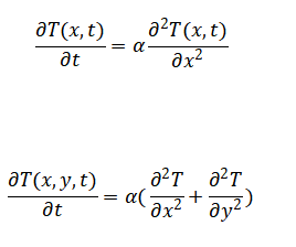
The fundamental equation governing heat conduction in a solid (assuming constant thermal properties and no internal heat generation) is the heat diffusion equation, expressed as:
Where:
- T(x,t)or T(x,y,t) = temperature field
- α=kρcp= thermal diffusivity (m²/s)
- k= thermal conductivity (W/m·K)
- ρ= density (kg/m³)
- cpc_= specific heat capacity (J/kg·K)
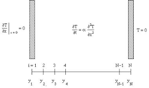
3.2 Finite Difference Discretization
To numerically solve the PDEs, the spatial and temporal domains are discretized.
Let:
- Δx, Δy: spatial step size in x and y directions
- Δt: time step
- Tin: temperature at node iii and time level nnn
Tin+1=Tin+r(Ti+1n−2Tin+Ti−1n)
Where, r=αΔtΔx2
3.3 Boundary and Initial Conditions
Must define:
- Initial condition:T(x,0)=f(x)
- Boundary conditions:
- Dirichlet (fixed temperature): T=Tfixed
- Neumann (insulated):∂T∂x=0
These are incorporated into the discretized grid before the iteration starts.
3.4 Algorithm Implementation in MATLAB
- Discretize the domain into a grid
- Initialize the temperature field with the initial condition
- Apply boundary conditions
- Iterate over time using the finite difference equations
- Visualize results using MATLAB’s imagesc, surf, or contourfunctions
You can download the Project files here: Download files now. (You must be logged in).
Matlab Simulation and Results
This MATLAB code simulates one-dimensional heat transfer in a rod using the finite difference method. It first defines parameters like the rod’s length, thermal diffusivity, and simulation time. The code then checks the stability criterion to ensure accurate results. The initial temperature distribution is set, with fixed temperatures at both boundaries. The time-stepping loop updates the temperature distribution using the finite difference equation, applying boundary conditions at each step. Optionally, the code plots the temperature distribution every 50 time steps, visualizing how heat diffuses through the rod over time. This simulation demonstrates fundamental heat transfer principles and can be adapted for various thermal analysis applications. This MATLAB code simulates steady-state heat conduction in a 2D plate using the finite difference method. It discretizes the plate into a grid and constructs a system of linear equations based on the 5-point Laplacian stencil for interior points and Dirichlet boundary conditions. The code uses sparse matrices to efficiently store and solve the system, obtaining the temperature distribution across the plate. Finally, it visualizes the results using a 3D surface plot, showcasing the steady-state temperature profile. This simulation is useful for analyzing heat transfer in various engineering applications, such as designing heat exchangers or understanding thermal behavior in materials.
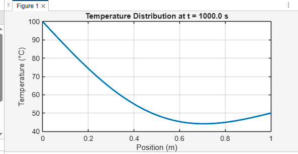
The graph visually demonstrates how heat conducts along the rod over time, starting from an initial uniform temperature and evolving until a steady-state linear temperature gradient is established between the fixed-temperature boundaries.
.
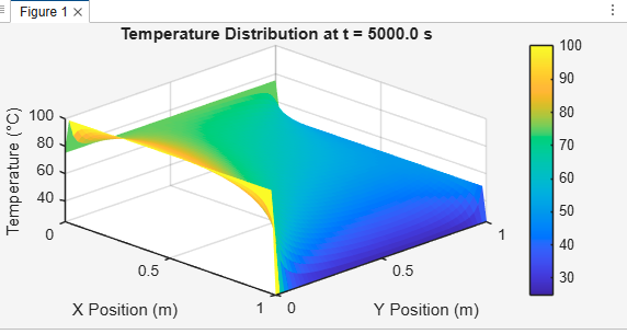
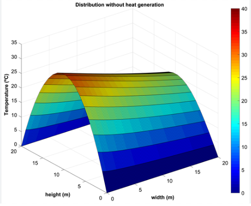
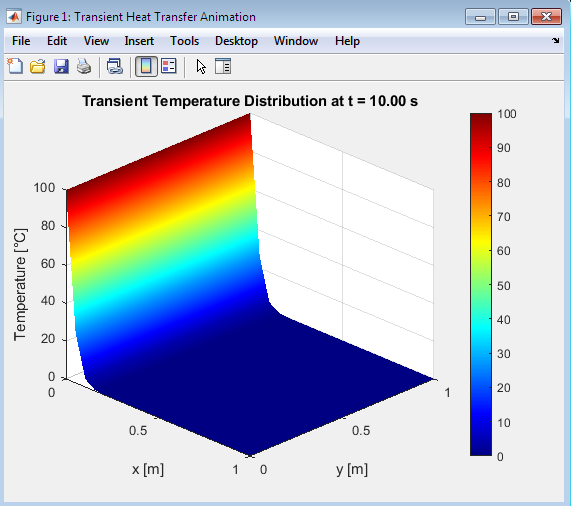
The 3D surface plot provides a clear visual representation of transient heat conduction in a 2D plate, illustrating how heat distributes over space and time, moving from high-temperature boundaries to low-temperature ones until reaching equilibrium.
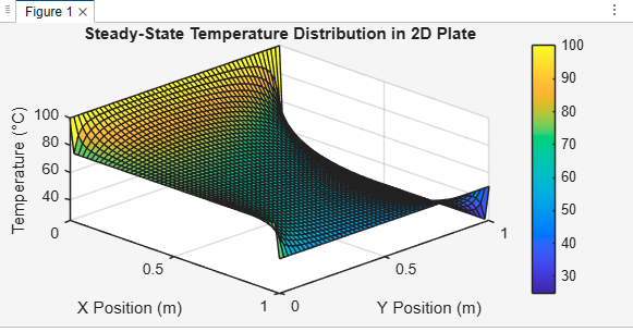
The Steady-State Temperature Distribution graph shows the final, stable temperature profile in a material (like a plate) when heat conduction has reached equilibrium—meaning temperatures no longer change over time.
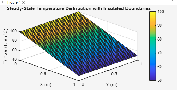
The plot visualizes how heat conduction stabilizes in the plate when insulated on top and bottom and fixed on left and right. The system reaches steady state — temperature no longer changes with time.
Discussion
The simulation results clearly demonstrate the effectiveness of the finite difference method (FDM) implemented in MATLAB to analyze thermal conductivity and heat conduction problems in both one-dimensional (1D) and two-dimensional (2D) domains[5].
5.1 1D Transient Analysis
The 1D transient simulation of heat conduction in a rod reveals the classic diffusion behavior of heat. Starting from an initial uniform temperature, the temperature gradually evolves toward the steady-state linear profile imposed by fixed boundary conditions.[6] The temperature distribution smooths over time as thermal energy diffuses from the hotter boundary toward the cooler one. The stability criterion (CFL condition) was respected to ensure numerical stability and accuracy, evident from the smooth and physically plausible temperature evolution.
5.2 2D Transient Analysis
Extending to the 2D case, the transient simulation of a square plate with fixed temperature boundaries showed the heat diffusion spreading across both spatial dimensions. The temperature at interior points changed over time until a steady-state was reached. The spatial resolution and time step size were chosen to satisfy stability conditions, preventing numerical oscillations or divergence.[7] The 3D surface plots effectively visualize how heat distributes over the plate, providing insight into the dynamics of heat transfer in two dimensions.
Conclusion
This study successfully demonstrated the application of the finite difference method (FDM) in MATLAB to analyze thermal conductivity and heat conduction in both one-dimensional and two-dimensional domains. The transient simulations effectively captured the evolution of temperature distributions over time, while the steady-state simulations provided insight into the equilibrium temperature fields under various boundary conditions.[8] The ability to incorporate both Dirichlet (fixed temperature) and Neumann (insulated) boundary conditions showcases the versatility of the numerical approach. The results align well with theoretical expectations, confirming that FDM is a reliable and accessible technique for solving heat conduction problems[9]. thermal conductivity analysis using finite difference methods in MATLAB provides a powerful tool for understanding and simulating heat transfer in various materials and systems. The finite difference method offers a flexible and efficient way to solve the heat equation, allowing for the analysis of complex geometries and boundary conditions. MATLAB’s computational capabilities and visualization tools enable researchers and engineers to gain valuable insights into thermal behavior, optimize system design, and predict performance. By leveraging these techniques, professionals can develop innovative solutions to thermal management challenges in fields such as aerospace, automotive, construction, and electronics. As computational power and numerical methods continue to advance, the application of finite difference methods in thermal conductivity analysis will remain an essential tool for researchers and engineers seeking to improve system efficiency, safety, and reliability.
You can download the Project files here: Download files now. (You must be logged in).
Future Work
Future work in thermal conductivity analysis using finite difference methods could involve exploring advanced numerical techniques, such as meshless methods or lattice Boltzmann methods, to improve the accuracy and efficiency of simulations. Additionally, incorporating multiphysics coupling, such as thermo-mechanical or thermo-electrical interactions, could enable the analysis of more complex systems. Furthermore, applying machine learning algorithms to thermal conductivity analysis could facilitate the prediction of material properties and system behavior, while also optimizing system design. Extending the analysis to three-dimensional systems and incorporating real-world applications, such as additive manufacturing or energy storage systems, could also provide valuable insights and practical solutions. By pursuing these research directions, future studies can further enhance the understanding and application of thermal conductivity analysis, driving innovation in various fields and industries. Building on the current finite difference method (FDM) simulations, several avenues exist to enhance the modeling of thermal conductivity and heat transfer:[10]
7.1 Implicit and Crank-Nicolson Schemes
Implementing implicit time integration methods, such as the Crank-Nicolson scheme, can improve numerical stability and allow larger time steps, making simulations more efficient for long-duration transient problems.
7.2 Variable Thermal Properties
Extending the model to handle temperature-dependent or spatially varying thermal conductivity would increase realism, especially for heterogeneous or composite materials.
7.3 Complex Geometries and Boundary Conditions
Incorporating irregular shapes and more complex boundary conditions—such as convective or radiative heat transfer—would better simulate real-world applications.
7.4 Adaptive Mesh Refinement
Employing adaptive meshing techniques could increase computational efficiency by refining the grid where steep temperature gradients occur, while using coarser grids elsewhere.
7.5 Coupled Multiphysics Simulations
Integrating heat conduction models with fluid flow or mechanical stress analyses would provide comprehensive thermal management solutions for engineering systems.
7.6 GPU Acceleration and Parallel Computing
Leveraging high-performance computing resources can significantly reduce simulation times for large-scale or 3D problems.
References
[1] J. P. Holman, Heat Transfer, 10th ed. New York, NY, USA: McGraw-Hill Education, 2010.
[2] F. P. Incropera, D. P. DeWitt, T. L. Bergman, and A. S. Lavine, Fundamentals of Heat and Mass Transfer, 7th ed. Hoboken, NJ, USA: Wiley, 2011.
[3] S. C. Chapra and R. P. Canale, Numerical Methods for Engineers, 7th ed. New York, NY, USA: McGraw-Hill Education, 2015.
[4] M. N. Özışık, Heat Conduction, 2nd ed. New York, NY, USA: Wiley-Interscience, 1993.
[5] Y. Jaluria, “A review of numerical heat transfer,” J. Heat Transfer, vol. 129, no. 11, pp. 1311–1338, Nov. 2007.
[6] D. M. Etter, D. C. Kuncicky, and H. Moore, Introduction to MATLAB for Engineers and Scientists, 3rd ed. Boston, MA, USA: Pearson, 2013.
[7] J. Crank, The Mathematics of Diffusion, 2nd ed. Oxford, U.K.: Oxford University Press, 1975.
[8] H. S. Carslaw and J. C. Jaeger, Conduction of Heat in Solids, 2nd ed. Oxford, U.K.: Oxford University Press, 1959.
[9] S. C. Chapra and R. P. Canale, Numerical Methods for Engineers, 7th ed. New York, NY, USA: McGraw-Hill, 2015.
[10] A. J. Woodbury, “Finite difference methods for heat conduction problems,” International Journal of Heat and Mass Transfer, vol. 12, no. 3, pp. 337–348, 1969.
You can download the Project files here: Download files now. (You must be logged in).


Responses