

Thermal Behavior Of Hydraulic Systems: Servo Hydraulic Actuator X Digital Electro Hydrostatic Actuator
Author: Waqas Javaid
Abstract
The pursuit of lighter, more efficient, and reliable flight control systems has motivated the exploration of alternatives to conventional Servo Hydraulic Actuators (SHA), which, although reliable, exhibit internal leakage and significant heat generation. In SHAs, small orifices in servo valves induce friction and convert pressure energy into heat, elevating fluid temperature and potentially impairing performance. Digital Hydraulics has emerged as a promising approach, employing parallel on/off valves to minimize losses and enhance efficiency. This study investigates the thermal performance of an SHA and a Digital Electro-Hydrostatic Actuator (DEHA), the latter integrating fixed-displacement pumps and a multi-chamber cylinder capable of 43 discrete velocity levels, achieving efficiency gains of up to 60%. Temperature estimation was performed using Carvalho’s (2023) algebraic thermal network model, adapted for steady-state analysis and validated through Hopsan and MATLAB/Simulink simulations. Results indicate that SHA valve temperatures exceeded 40 °C, whereas all DEHA nodes remained near the 20 °C ambient level, evidencing reduced heating and improved efficiency.
1. Introduction
Hydraulic valves used in aircraft are fast and reliable, however, they suffer from internal leakage (NOSTRANI, 2021). Pressure drops caused by throttling of the fluid and internal leakage make actuation systems present low energetic efficiency. On aircraft, pressurized fluid is used to promote the movement of many different components. The aerospace sector, on which aeronautical engineering is included, has an important role in technological development. Despite regular flight being achieved in the last century, research on fluid power is necessary for the maintenance and betterment of this technology. There is a constant need for innovation in the industry, ever reaching for lower costs, less mass and for improvements in efficiency, reliability and safety.
In 2007, aviation was responsible for transporting over 2.5 billion passengers/year and over 50 million tons of payload, transporting up to 35% of global trade value. Not only that, but it is also responsible for over 15 million jobs, plus estimated 16 million tourism jobs made possible by aviation. It has a turnover of U$1 trillion and 145% growth expected between 2007 and 2026. (OXFORD ECONOMICS, 2011). Fluid power is ideal for high speed, high force, high power applications, being unsurpassed for force and power density compared to all other actuation technologies, capable of generating extremely high forces with relatively lightweight cylinder actuators. (DURFEE et. al, 2015). On aviation, fluid power is used in many important systems, including primary and secondary control surfaces, landing gears, cargo doors and steering systems (WARD, 2017). The main topology used for that is Servo-Hydraulic Actuators – SHA, present on both civil and military aircraft, such as: Airbus A320, A380, Boeing B787, and fighter aircraft like McDonnel Douglas F15 and Lockheed Martin F16 (WANG, 2012). However, due to its low efficiency caused by the dissipative control of throttling the flow through control orifices and by losses due to the leakage of oil at connections and seals, research is being done to replace or complement aircraft hydraulic actuators with other types of systems. One such concept is that of More Electric Aircraft – MEA (BENNETT et al., 2010; CAO et al., 2012; NAAYAGI, 2013), which aims to replace pneumatic, hydraulic and mechanical actuation with electric actuators, which are highly efficient (BOZHKO, S., HILL, C. I. & YANG, 2018) and are already in use by some types of aircraft (MOOG, 2018). Even so, the designs developed often still use hydraulic systems, as is the case on Electro-Hydrostatic Actuator – EHA, and the reliability of conventional SHA systems is difficult to surpass.
A new line of research focused on improving the efficiency of hydraulic systems has been gaining space in the academic community in the last few years, called Digital Hydraulics (UUSITALO et al., 2009; WINKLER et al., 2010; NOSTRANI, 2015; NOSTRANI et al., 2017). In digital hydraulic systems, the control of flow rate and pressure is performed to reduce the main energy losses. The results have been promising, with an increase in around 60% efficiency compared to traditional solutions (Dell’ Amico et al, 2013, Linjama et al., 2009). More recently, in Belan (2018), Nostrani (2021) and Silva (2023), three digital hydraulic actuators were presented, with an equivalent performance and efficiency reaching 30 times that of conventional solutions. The Brazil-Sweden partnership between LASHIP-UFSC, FLUMES-LIU, CERTI and SAAB AB has been showing promise on digital hydraulic systems applied on aerospace. It has resulted in three doctoral theses and four master’s theses.
As research is done to increase efficiency, systems may become smaller and lighter, allowing for bigger payloads, drag reduction and fuel savings. However, while this optimization brings many advantages, one of its downsides is that with their dimensions reduced the thermal effects of fluid flow become more significant. When oil passes through small orifices, such as that of servo valves, there is an increase in the temperature due to friction and the conversion of pressure energy into thermal energy inside the system’s components. In some cases, the excessive heat can eventually compromise the equipment’s performance and damage its internal components. Despite this, few literature studies seek to analyze flight control systems’ dynamics and thermal effects (PINTARELLI, 2022), and there is a lack of modeling techniques of hydraulic fluid power systems that allows designers to determine the temperature on steady flow with low computational cost and without missing temperature data of components (CARVALHO, 2023).
To evolve in the design of digital hydraulic systems, it is necessary to better comprehend thermal effects on digital hydraulic systems and how they compare to traditional solutions, what design changes it allows and how it may affect different aircraft systems, such as the Flight Control Systems – FCS.
1.1. Main Objectives
The main objective of this study is to determine the thermal behavior and effects of temperature in steady-state on conventional aircraft flight control systems (SHA) and how it compares to the emergent technology that is digital hydraulics, in special the Digital Electro Hydrostatic Actuator (DEHA). To do that, simulations will be performed to acquire data that can then be used on an algebraic mathematical model of temperature prediction of hydraulic systems.
1.2. Specific Objectives
- To compare the DEHA with a standard SHA fluid power solution.
- To perform numerical simulations of the SHA and DEHA circuits and obtain relevant parameters such as pressure and fluid flow values in distinct points.
- To apply an algebraic mathematical model of temperature prediction of hydraulic systems to determine temperature in relevant hydraulic components.
- To verify difference in size of heat exchangers according to temperatures obtained and conditions analyzed.
2. Literature Review
2.1. Fundamentals of Flight and Aerodynamics
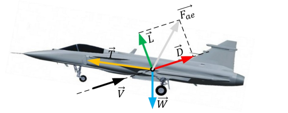
Four basic forces are involved on aircraft flight: Thrust , drag , lift and weight . Lift and drag are components of the Aerodynamic Force and are caused by the relative movement between the aircraft and the air surrounding it, while the thrust force is provided by the engines and weight is a result of the gravitational force in response to the aircraft’s mass. (HOEKSTRA, 2021). In Figure 1 these vectors can be seen.
Source: Rodrigo Simão Lopes, adapted from Ribeiro (2018).
For constant speed and altitude, force equilibrium shows that lift is equal to weight and thrust is equal to drag.
Lift is mainly generated by the wings, with a small contribution of the horizontal tail plane. The weight is composed of three main components, those being: the aircraft’s empty weight, its fuel and its payload. The thrust force is provided by the engines to counteract the drag, caused by friction between the aircraft surfaces and the air surrounding it. During takeoff and landing, a higher lift force is needed as the aircraft is flying at low speed. For that, devices are used to increase the lift coefficient and wing area, S. Highlighted on Figure 2, there are flaps located at the back of the wings (used during both takeoff and landing), and slats/leading edges, highlighted on Figure 2, on the front are used during landing. (HOEKSTRA, 2021).
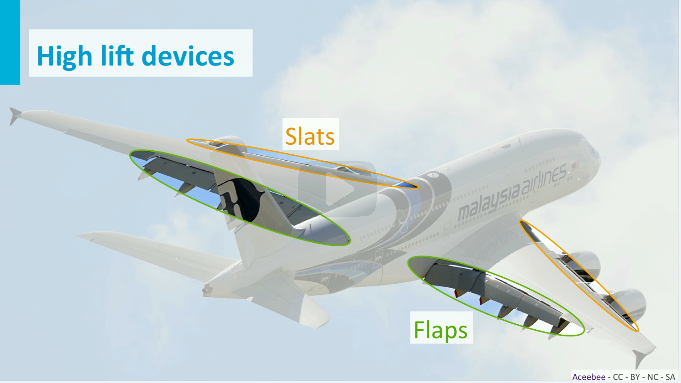
Source: Aceebee, adapted by TU Delft (2017).
Stability and control of aircraft is still a hard problem, and interaction between pilot and machine in the form of Pilot Induced Oscillations – PIO remains problematic. There are four controls in which the pilot can control the direction of flight, those being: Thrust (forward acceleration and hence forward speed), ailerons (to control the bank angle and control the aircraft), elevator (controls the nose up and down, pitch), rudder (controls yawing movement, where the aircraft is leading). To control these and other important aircraft systems, flight control surfaces are used. (HOEKSTRA, 2021).
2.2. Flight Control Surfaces
Control surfaces may be classified in two main groups: primary and secondary control surfaces. Primary control surfaces are responsible for controlling the flight route and are composed of the ailerons, elevators and rudders (FAA, 2016), as highlighted on Figure 3 – Primary control surfaces of a typical aircraft Figure 3.
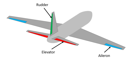
Source: Pintarelli (2022).
Secondary control surfaces, such as wing flaps, leading-edge devices (e.g, slats), spoilers and trim systems, reinforce the action of primary control surfaces, improve the aircraft’s flight characteristics and reduce excessive control forces (FAA, 2016).
2.3. Aircraft Control Actuators
The control of flight surfaces is done through an actuation system, which can be comprised of different topologies. The most applied are: Electro-Mechanical Actuators – EMA, Servo Electro-Hydraulic Actuators – SHA, and Electro-Hydrostatic Actuators – EHA.
2.3.1. Electro-Mechanical Actuators – EMA
An electro-mechanical actuator (EMA) converts electrical energy into mechanical energy to control the motion of a mechanical system. It can provide precise motion control by combining a DC brushless electric motor and a gearbox (MOIR & SEABRIDGE, 2008).
According to Wang et. al (2016), some of its advantages include:
- Reduce flight control weight by 25%.
- Reduce maintenance by 42%.
- Reduce the meantime repair by 50%.
- Increase aircraft availability.
However, according to the same authors, it has two main disadvantages: the possibility of the actuator jamming, in which case it is unable to move either due to mechanical or electrical issues, and its size. Jamming can be prevented or mitigated through proper maintenance and careful monitoring of the actuator’s performance
2.3.2. Servo Electro-Hydraulic Actuators – SHA
May be powered by aircraft engines or consist of an electric motor that drives a hydraulic pump, which powers a hydraulic cylinder or motor. They are used in some of the most important systems of modern aircraft, including the control of primary and secondary flight control surfaces (MOIR & SEABRIDGE, 2008), landing gears, cargo doors, steering and others. (WARD, 2017)
One of its main disadvantages comes from the use of servo valves, that despite being fast and reliable present internal leakage and pressure drops that result in energy losses. (NOSTRANI, 2021). In Figure 4, it is possible to observe the functioning of a mechanical hydraulic actuator.
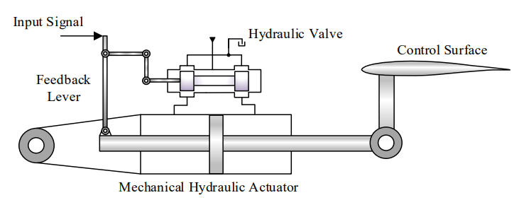
Source: Nostrani (2021), adapted from Wang et. al (2016).
It consists of a mechanically signaled, hydraulically powered actuator equipped with an integrated feedback mechanism and supplied by a centralized hydraulic power unit (HPU). The control input, typically derived from a pilot-operated lever or mechanical linkage, displaces a directional control spool valve connected to the high-pressure hydraulic circuit. This displacement directs pressurized fluid into one side of a double-acting actuator while simultaneously venting the opposite chamber to the return line, producing linear motion that is transmitted to a control surface. A mechanical feedback linkage, coupled to the actuator rod, progressively re-centers the valve spool as the commanded displacement is achieved, thereby interrupting fluid flow and maintaining the control surface in its target position. This closed-loop arrangement minimizes pilot workload, ensures positional accuracy, and provides inherent stability by automatically compensating for external disturbances without requiring continuous manual correction. (NOSTRANI, 2021).
2.3.3. Electro-Hydrostatic Actuators – EHA
Topology of actuator that uses an electric motor to drive a hydraulic pump, which in turn powers a hydraulic cylinder or motor to produce mechanical movement. One of its main advantages is the substitution of systems that use a centralized power unit to one that has decentralized ones. According to Rongjie et al. (2009), three main EHA arrangements exist: A configuration with variable rotational frequency electric motor and fixed displacement pump (FPVM), another with fixed rotational frequency electric motor and variable displacement pump (VPFM) and lastly one with variable displacement pump/variable electric motor (VPVM), as seen on Figure 5.
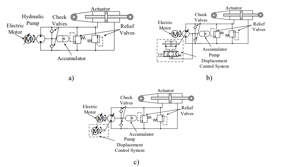
Source: Nostrani (2021), based in Alle et al. (2018) and Wang et al. (2016).
2.4. Digital Hydraulic Systems
The objective of digital hydraulic systems is to propose and provide energy efficient alternatives, though its precise definition is still a topic of discussion among researchers (ACHTEN et. al, 2013). According to Linjama (2011), digital hydraulic systems can be defined as hydraulic systems that contain discrete components, capable of actively controlling the output of the system.
The goal of these systems is to increase energetic efficiency through the reduction of resistive and dissipative effects in flow and pressure control. According to Scheidl et al. (2012), digital hydraulics has considerable advantages when compared to traditional alternatives, such as high efficiency, robustness and high capacity for the standardization of components. As mentioned in the introduction, there were instances in which an increase of up to 60% in efficiency was achieved when compared to conventional solutions. (DELL’ AMICO et al., 2013, LINJAMA et al., 2009).
In Belan (2018), Nostrani (2021) and Silva (2023) three digital hydraulic actuators were presented, with equivalent performance and efficiency reaching up to 30 times that of conventional solutions.
As shown in Table 1, digital hydraulics can be applied in all units of a hydraulic system, being its solutions based on two modes of operation: parallel associated elements or fast switching (LINJAMA, 2011). The behavior of parallel systems can be determined by the contribution of hydraulical components, including valves, with their size and quantity resulting on a given flow control, as well as pumps, actuators and hydraulic motors. Fast switching makes use of one or more valves, controlled with the technique of Pulse-Width Modulation – PWM, with the control flow depending on the width and frequency of the switching pulses.
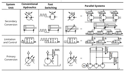
Source: Rodrigo Simão Lopes, based in Linjama (2011), Belan (2018), Nostrani (2021). Translated by author.
Both concepts rely on on/off valves to ensure proper performance. For these applications, seat valves are the most used. This variant of valve is characterized by its ease of manufacture, strong resistance to heat and contaminants and minimal internal leakage, making for a highly reliable component, with a rate of failure in the order of (BELAN, 2018; LINJAMA, 2011; MANTOVANI, 2019; PETTERSSON, 2018). Its main components are in Figure 6.
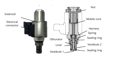
Source: Mantovani (2019), translated by author.
Some counterpoints include (LINJAMA, 2011; ACHTEN, et al., 2013):
- High level of noise.
- Elevated pulse pressure.
- Nonconventional control techniques.
- Larger components.
- Low durability and life, due to the high frequency of commutation.
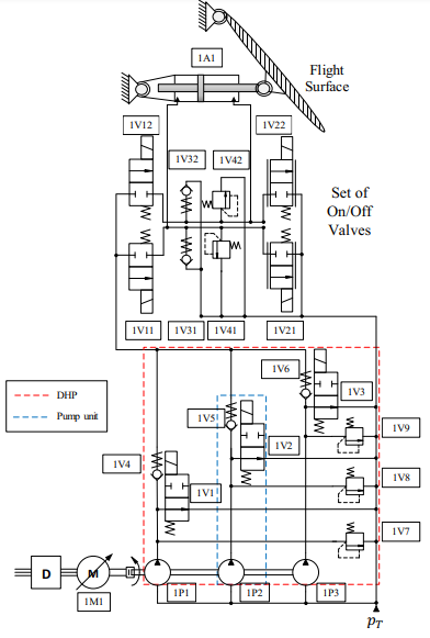
The Brazil-Sweden partnership between LASHIP-UFSC, FLUMES-LIU, CERTI and SAAB AB has been showing promise on digital hydraulic systems applied on the actuation of primary control surfaces, and so far, has resulted on three doctoral theses and four master’s theses. Up to the publication of this bachelor thesis, three digital actuator designs aimed at FCS were developed as part of this partnership, on doctoral level research of Belan (2018), Nostrani (2021) and Silva (2023). Belan’s solution, the Digital Hydraulic Actuator (DHA) uses secondary control on a multichambered actuator and multiple pressure supply lines, which are connected to on/off valves instead of Digital Flow Control Units – DFCUs. It utilizes a central hydraulic unit with three distinct pressure level lines, four different areas of a multichambered cylinder and 12 on/off valves, totaling 81 discrete forces used to control the position of the actuator. Belan demonstrated a reduction on energy dissipation ranging between 80% and 93% when comparing the DHA to the standard SHA on evaluations using typical inputs on a single aileron from the aircraft model “F16systemManeuver”. This model is available on Hopsan®, a free simulation environment for fluid and mechatronic systems, developed at Linköping University. The DHA is shown in Figure 7.
Source: Belan (2018), translated by author.
Other studies were made to better evaluate the capabilities of the DHA. Ward (2017) applied the DHA to all ailerons of the model “F16systemManeuver”, which resulted in a 30% reduction on the consumption of hydraulic power. Dell’Amico et al. (2018) tested the performance of the DHA on the internal elevons in the model “ADMIRE”, reducing the hydraulic power used by 40%. Cruz (2018) compared the DHA to a SHA model with real internal leakage data of a servo valve, concluding that the DHA presented up to 30 times less dissipated energy.
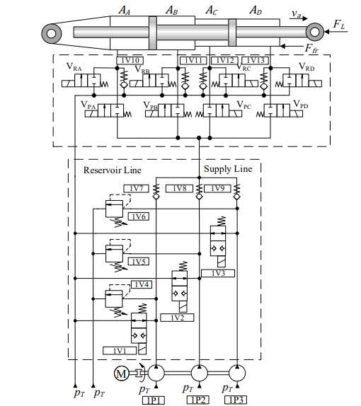
Another solution, proposed by Silva (2023) is a configuration of hydraulic actuator that combines the benefit of the MEA concept with Digital Hydraulics, composed of a decentralized actuation system with an electric motor with speed control and a digital hydraulic pump (DHP) to move a symmetric actuator. It also replaces the use of servo valves with on/off valves, reducing the weight of the system and making it more flexible to new arrangements, as can be seen in Figure 8.
Source: Silva (2023).
You can download the Project files here: Download files now. (You must be logged in).
The use of a variable speed digital pump applies the power-on-demand concept, aiming to control the hydraulic energy supplied to the system, and the DHP increases the number of different flow rates provided at each rotational frequency, optimizing the use of the pump through more efficient combinations (SILVA et al., 2021). The VSDEHA can also be applied to a multichambered cylinder.
Experiments were done on a test bench to validate the concept, with an energetic evaluation reaching up to 58% efficiency on the conversion of hydraulic energy to useful energy output in the cylinder. Simulations compared the VSDEHA to other actuators. Compared to an EHA, it achieved twice the efficiency in converting hydraulic energy, and when compared to a SHA in a flight simulation, the VSDEHA needed about 22 times less energy to perform the same work. (SILVA, 2023).
2.4.1. Digital Electro Hydrostatic Actuator – DEHA
The solution proposed by Nostrani, named Digital Electro Hydrostatic Actuator – DEHA, shown on Figure 9, is based on techniques of primary and secondary control. Making use of a decentralized hydraulic power unit – DHPU, and three fixed displacement pumps that make up eight possible volumetric displacements, associated to a multichambered cylinder with four distinct areas, is capable of operating on either normal or regenerative mode, totaling six equivalent areas and 43 discrete levels of velocity. Through mathematical modeling, simulations and experimental data, Nostrani concluded that the DEHA consumes 31 times less energy than the SHA and 1.7 times less than the EHA, technologies typically used for flight control surfaces (NOSTRANI et al., 2020).
Source: Nostrani (2021).
2.5. Thermo-hydraulics
There are few academic references on the impact of temperature on flight control system’s components. (PINTARELLI, 2022). The increase in temperature, however, is not always negligible due to conversion of pressure energy into thermal energy when the working fluid goes through small orifices, such as damping orifices or inside electrohydraulic servo valves (EHSV). Depending on the increase of temperature of the working fluid, the excessive heat may eventually compromise the performance of the system as well as damage its internal subcomponents. Thus, the study of hydraulic flow in thermal fluids is important for the safety and advancement of this field and that is the aim of thermohydraulics. It can be divided in three parts: fluid mechanics, thermodynamics and heat transfer, even though they are all coupled (AKIMOTO et al., 2016). Fluid mechanics deals with the behavior of fluids at rest and in motion (FOX et al., 2004), governed by definitions and fundamental equations such as flow velocity, pressure gradient, buoyancy, Bernoulli’s equation, Euler equations and Navier-Stokes equations, among others; Thermodynamics is the study of energy and its interactions of a system with its surroundings, by work and heat, using the end states of a process. Heat transfer extends thermodynamic analysis through the study of modes of heat transfer, those being conduction, convection and radiation, with relations to calculate heat transfer rates. (INCROPERA et al., 2011). It summarizes the process of exchanging energy and cooling performance of components (PINTARELLI, 2022).
To compare the temperature between the conventional SHA and the digital hydraulic solution entitled DEHA, simulations are performed using the softwares MATLAB/Simulink and Hopsan to obtain parameters and acquire data that can then be used on the algebraic mathematical model of temperature prediction of hydraulic systems developed by Carvalho (2023).
2.5.1. Algebraic mathematical model for temperature prediction of hydraulic systems
The common approach for hydraulic analysis is the design of a dynamic model with parameters on numerical simulation softwares, aiming for an optimized relation between computation cost and precision. To include the dynamic of temperature for each control volume, however, significantly increases the computational cost, not adequate in the first design stages of systems, where a great number of simulations are required. Steady-state models can be used to go around this limitation, which simplifies models at the cost of reducing the number of control volumes and thus of places where the temperatures are known. (CARVALHO, 2023). For this reason, in his master level thesis, Carvalho proposed the adaptation of algebraic mathematical modeling used in district heating networks (WANG et al., 2016) to hydraulic systems. With the simplification of hydraulic components into two basic elements, branches and nodes, the author proposed a new matrix-based simulation model that enables rapid resolution of steady-state thermal simulation models through matrix operations, while also facilitating the addition or modification of components in an existing model. To adapt the method developed by Wang et. al (2016), changes were made to the energy balance originally proposed, as the heating of hydraulic components is due to pressurization, viscosity and friction. The pump, for instance, transforms part of the energy received from its surroundings into temperatures through the phenomena of friction and through internal leakage, which transfers the fluid with more energy at the pressurized line to suction, where the energy contained in the fluid will in time transform into temperature due to viscosity (CARVALHO, 2023).
This thermal analysis consists of applying the Conservation of Energy to the different elements of a thermal network. For that, understanding the dynamic modeling of a hydraulic system with concentrated parameters is useful since the same topology is used for prediction within the algebraic model.
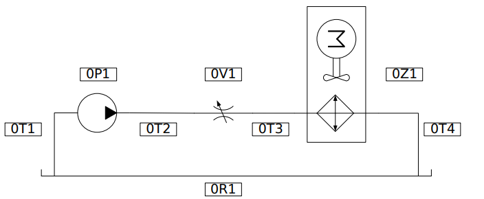
Considering as an example the following hydraulic system, represented in Figure 10, containing: Pump (0P1), valve (0V1), heat exchanger (0Z1) and reservoir (0R1). The pump receives mechanical energy in the form of work () and converts part of this energy into enthalpy ( in the fluid that goes through the component. The valve does not perform work, but dissipates part of the hydraulic energy received from the pump and produces entropy. The heat exchanger dissipates hydraulic energy while also exchanging heat ( into the system surroundings.
Source: Carvalho (2023).
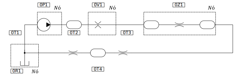
For this system, the standard approach is to admit that the pump (0P1) operates on steady flow, since its internal volume is small in comparison to the other components in the system, and since its transient period is significantly smaller than that of the heat exchanger (SIDDERS et al., 1996). On such case, it is convenient to admit that the pump is a flow source connected to a control volume that represents the pipes/conduit (0T2). The same approach can be taken for the valve (0V1), though the model now used is that of a flow restriction followed by a control volume. For the heat exchanger the interpretation is different, making use of a restriction that reproduces the loss of hydraulic energy given a volumetric flow between its inlet and outlet, in addition to a control volume that represents it, and thus the restriction control volume is the same component. (CARVALHO, 2023). Figure 11 illustrates a closed-loop hydraulic circuit designed for the actuation of a double-acting cylinder. Fluid is drawn from the reservoir (0R1) through the suction line (0T1) into the hydraulic pump (0P1), which pressurizes the flow. The pressurized fluid passes through a line filter (0T2) to remove contaminants before entering a check valve (0V1) that ensures unidirectional flow toward the actuator. A second filter or coupling element (0T3) further conditions the fluid before it reaches the double-acting hydraulic cylinder (0Z1), where hydraulic energy is converted into linear motion. The return flow from the actuator travels through the return line (0T4), passing another filtering stage, and is discharged back into the reservoir (0R1), completing the cycle. This configuration ensures continuous operation with controlled flow direction and efficient conversion of hydraulic power into mechanical work.
Source: Carvalho (2023).
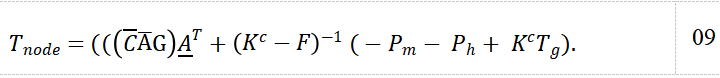
According to Carvalho (2023), it is possible to prove that for a control volume with multiple inlets and oulets, the following equation is valid:
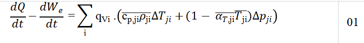
In which is the difference in temperature, the difference in pressure, from the outlet in relation to the inlet at the control volume, is the volumetric flow through a control volume, (1/K) is the modular average coefficient of isobaric volumetric expansion, is the average temperature, is the heat transfer rate through the control surface and is power exchanged from the system and its surroundings, with the heat flux being positive when the system receives heat, and power is positive when work is done by the control volume. For a network of branches (pipes, heat exchangers, valves) connected at nodes (reservoirs, junctions), the code is based on steady-state nodal thermal–hydraulic balancing, where the energy balance at every node is adapted from the First Law of Thermodynamics (CARVALHO, 2023). Thus Equation 01 can be adapted into:
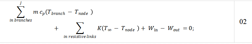
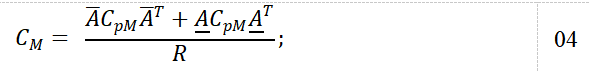
In Equation 02 above, is the mass flow rate, the specific heat capacity, the heat transfer coefficient and thermal power. The relationship between nodes and branches are established using positive and negative incidence matrices ( and can be used to form the nodal normalization matrix, (CARVALHO, 2023):
![]()
normalizes the conductance and capacity matrices and counts the number of connections to each node, and is used to form the nodal capacity matrix, indicated by Equation 04:
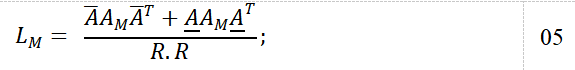
These terms are used to form the nodal area/inertia matrix:
in which The pressure-flow power term is then given by:

Where is the diagonal matrix of flow rates, presents pressure at each node and “1” is a column vector of ones. For the calculation, terms are combined in the flow coupling matrix :
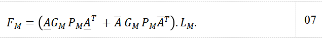
Combining all equations together, it is possible to obtain an equation for the system, a matricial form equation containing the steady-state nodal temperature, with an initial reference of ambient temperature .
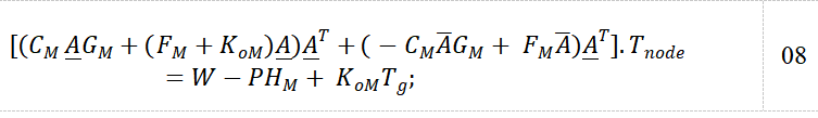
The final solution comes from isolating the nodal temperatures. In analytical form, the prediction of steady-state temperature can be represented with Equation 09:
3. Methodology
This chapter presents the procedures and methods used for the making of this bachelor thesis, as well as the application of the literature review presented. The thermal analysis was separated in steps, since two different topologies (SHA and DEHA) were compared. First, the initial conditions of analysis were established, that being a steady-state regime with some known parameters and some obtained by numerical simulations. Before running the simulations, thermal models were defined for the SHA and DEHA, considering the elements of each system where heat and power dissipation are relevant. Then, numerical simulations were performed in MATLAB/Simulink with the SHA and DEHA models to obtain pressure and flow values at each relevant node and branch. After this, the thermal models were solved using the algebraic method developed by Carvalho (2023), to obtain temperatures at each node.
3.1. Initial Conditions of Analysis
The case examined is that of an actuator at rest during cruise with a load of 10.000 N, on which no fluid flows into or out the cylinder, but the pump still works and dissipates heat. The geometric parameters are relevant and already considered in the Hopsan and MATLAB models, as the flow and pressure values obtained are in function of them. Changing these parameters and exploring different solutions would give different results for pressure and flow values.
3.2. Servo Hydraulic Actuator – SHA Model
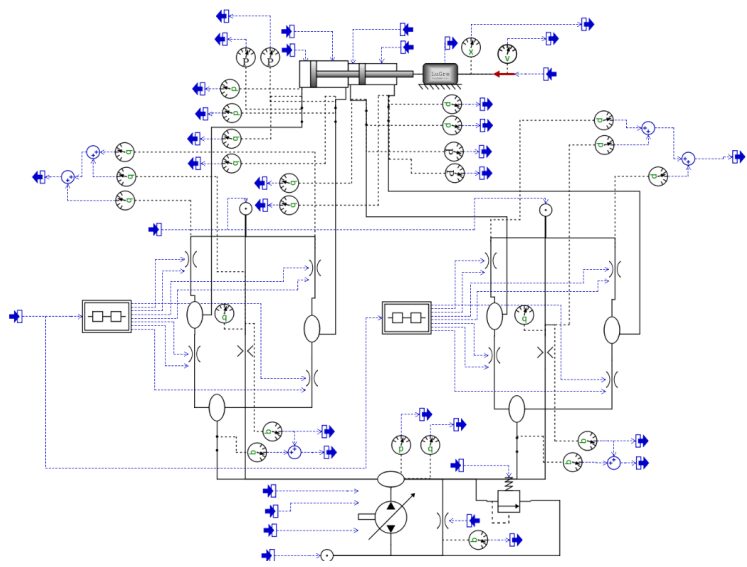
To obtain data for the thermal analysis, an existing SHA model is used on Hopsan. The model, as seen in Figure 12 consists of a four-chamber hydraulic cylinder (1A1), two servo valves (1V2, 1V3), a variable displacement pump (1P1), a fixed rotational frequency electric motor (1M1) and a relief valve (1V1).
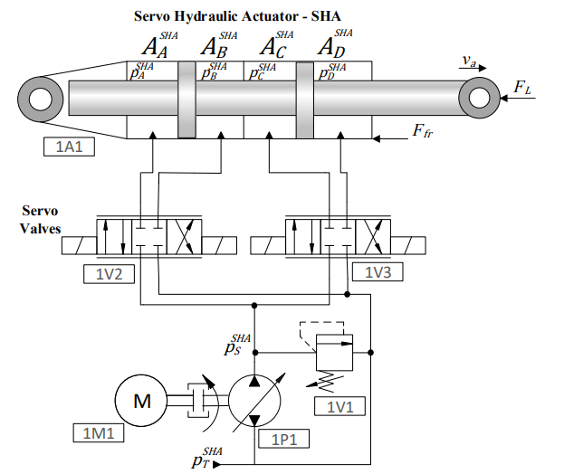
Source: Nostrani (2021).
The main parameters used for the SHA model in Hopsan are displayed in Table 2.
Table 2 – SHA Parameters
| Parameters | Value | Unit |
|---|---|---|
| A_A, A_B, A_C, A_D | 453.55 | mm² |
| l | 0.2 | m |
| β | 1.3 × 10⁹ | Pa |
| D_pv | 6.15 × 10⁻⁶ | m³/rot |
| p_rSHA | 10 × 10⁵ | Pa |
| w_npSHA | 125.66 | rad/s |
Source: Nostrani (2021).
In Hopsan, the model is represented as seen in Figure 13.
Source: Nostrani (2021)
This model is then imported to MATLAB, where it can be accessed via Simulink in the manner where its parameters such as pressure and flow values can be obtained.
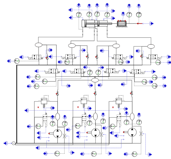
3.3. Digital Electro Hydrostatic Actuator – DEHA Model
Similarly, the DEHA that was shown in Figure 9 has its own Hopsan model imported into Simulink. In Figure 14, it is possible to see the three pumps connected to the reservoir, the relief valves, and the three main valves connected to the multi-chambered actuator. Its main parameters are shown in Table 3.
Table 3 – DEHA Parameters
| Parameters | Value | Unit |
|---|---|---|
| A_A | 47.9 × 10⁻⁴ | m² |
| A_B | 12.86 × 10⁻⁴ | m² |
| A_C | 10.71 × 10⁻⁴ | m² |
| A_D | 45.84 × 10⁻⁴ | m² |
| l | 0.2 | m |
| β_e | 1.3 × 10⁹ | Pa |
| B | 0.1 | Ns/m |
| V_OA | 6.8 × 10⁻⁵ | m³ |
| V_OB | 6.9 × 10⁻⁵ | m³ |
| V_OC | 6.8 × 10⁻⁵ | m³ |
| V_OD | 7.0 × 10⁻⁵ | m³ |
| C_LAB, C_LBC, C_LCD | 1 × 10⁻¹⁶ | m³/(s·Pa) |
Source: Nostrani (2021).
You can download the Project files here: Download files now. (You must be logged in).
3.4. Numerical Simulations
Fluid flow values and pressure values were obtained by using the Simulink models of the SHA and the DEHA. For each 80 seconds of simulations 1000 values were obtained. In order to simulate a steady-flow system, the first 20 seconds of simulation were discarded, as part of that data is when the system is not stabilized.
3.4.1. SHA Simulation
From the SHA simulation, the average of the following variables were taken from the last 60 seconds of simulation, using 10.000 N:
Table 4 – SHA Simulation Data
| Parameters | Value | Unit |
|---|---|---|
| p₀ | 1 × 10⁶ | Pa |
| p_s | 2.1 × 10⁷ | Pa |
| p_T | 2.1 × 10⁷ | Pa |
| p_r | 1 × 10⁶ | Pa |
| p_A | 4.40 × 10⁶ | Pa |
| p_B | 1.626 × 10⁷ | Pa |
| p_C | 4.40 × 10⁶ | Pa |
| p_D | 1.626 × 10⁷ | Pa |
| q_vA | -3.54 × 10⁻⁹ | m³/s |
| q_vB | 4.42 × 10⁻⁹ | m³/s |
| q_vC | -4.72 × 10⁻⁹ | m³/s |
| q_vD | 3.527 × 10⁻⁹ | m³/s |
| q_vP | 4.676 × 10⁻⁵ | m³/s |
Used as inputs for the thermal analysis are the already known pressures at the reservoir of 10 bar and the supply pressure of 210 bar , which is also the pressure at the pump, relief valve and T-junction.
3.4.2. DEHA Simulation
Similarly, the DEHA simulation yielded the average of the following variables, taken from the last 60 seconds of simulation, can be seen on Table 5:
Table 5 – DEHA Simulation Data
| Parameters | Value | Unit |
|---|---|---|
| P_pump,1 | 1.016 × 10⁶ | Pa |
| P_pump,2 | 1.0072 × 10⁶ | Pa |
| P_pump,3 | 1.0162 × 10⁶ | Pa |
| q_v,pump1 | 2.499 × 10⁻⁵ | m³/s |
| q_v,pump2 | 3.999 × 10⁻⁵ | m³/s |
| q_v,pump3 | 5.998 × 10⁻⁵ | m³/s |
| q_v,1 | 3.072 × 10⁻⁵ | m³/s |
| q_v,2 | 5.363 × 10⁻⁵ | m³/s |
| q_v,3 | 8.828 × 10⁻⁵ | m³/s |
| q_v,v1 | 2.495 × 10⁻⁵ | m³/s |
| q_v,v2 | 3.995 × 10⁻⁵ | m³/s |
| q_v,v3 | 5.991 × 10⁻⁵ | m³/s |
| P_VP,A | 1.10 × 10⁷ | Pa |
| P_VP,B | 1.10 × 10⁷ | Pa |
| P_VP,C | 1.10 × 10⁷ | Pa |
| p_VP,D | 1.10 × 10⁷ | Pa |
| q_v,vPA | -1.014 × 10⁻⁸ | m³/s |
| q_v,vPB | 0 | m³/s |
| q_v,vPC | -5.097 × 10⁻⁸ | m³/s |
| q_v,vPD | 0 | m³/s |
| q_v,vRA | 0 | m³/s |
| q_v,vRB | 8.533 × 10⁻⁹ | m³/s |
| q_v,vRC | 0 | m³/s |
| q_v,vRD | 1.003 × 10⁻⁸ | m³/s |
Source: Author.
3.5. Thermal Analysis
The thermal analysis is done using the algebraic mathematical model of temperature prediction of hydraulic systems. Hydraulic components are presented as nodes when thermal effects are relevant, and the fluid flow across the hydraulic circuit follows the path presented by branches. For that, in the last section the fluid flow and pressures were collected in specific points.
3.5.1. SHA Thermal Analysis
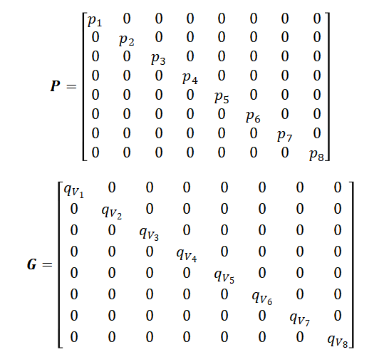
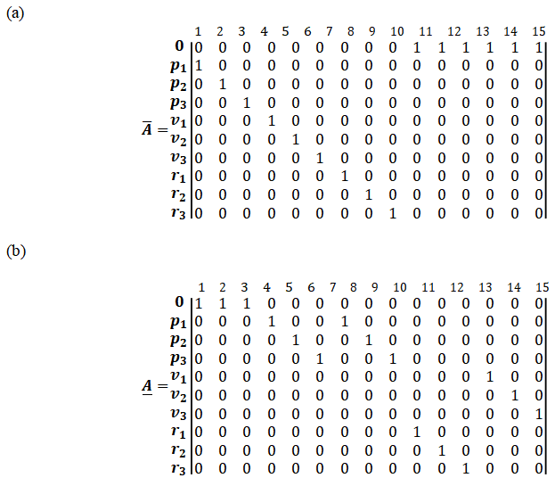
The SHA thermal model can be seen on Figure 15 and consists of a reservoir (), a pump (), a T-junction () and two directional valves () and an actuator with two servo valves (). The oil is pumped from the reservoir to a T-junction, which leads to a relief valve, a hydraulic actuator or to the cylinder. For thermal analysis, matrices are built based on the model presented below, which does not consider the relief valve nor the actuator, as thermal effects were negligible for the analysis.
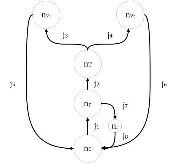
Source: By the author.
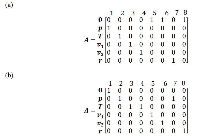
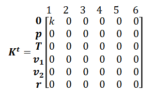
The incidence matrices are 6×8 (due to having 6 nodes and 8 branches) as represented in Figure 16:
SHA pressure data can be seen in Table 6, with 10 bar at the reservatoir, a supply pressure of 210 bar and an estimated drop of 1 bar after each valve.
Table 6 – SHA Pressures Data for Thermal Model on branches
| Parameters | Value | Unit |
|---|---|---|
| p₁ | 1 × 10⁶ | Pa |
| p₂ | 210 × 10⁵ | Pa |
| p₃ | 209 × 10⁵ | Pa |
| p₄ | 209 × 10⁵ | Pa |
| p₅ | 1 × 10⁶ | Pa |
| p₆ | 1 × 10⁶ | Pa |
| p₇ | 209 × 10⁵ | Pa |
| p₈ | 1 × 10⁶ | Pa |
Source: By the author.
Flow values for each branch were obtained from Simulink, with the averages being represented in Table 7.
Table 7 – SHA Flow Data for Thermal Model on branches
| Parameters | Value | Unit |
| qv₁ | 8.39 X 10⁻⁵ | m³/s |
| qv₂ | 4.26 X 10⁻⁵ | m³/s |
| qv₃ | 2.13 X 10⁻⁵ | m³/s |
| qv₄ | 2.13 X 10⁻⁵ | m³/s |
| qv₅ | 2.13 X 10⁻⁵ | m³/s |
| qv₆ | 2.13 X 10⁻⁵ | m³/s |
| qv7 | 4.13 X 10⁻⁵ | m³/s |
| qv₈ | 4.13 X 10⁻⁵ | m³/s |
On matricial form, they are represented in Figure 17.
Source: By the author.
For thermal effects, it is also important to consider the specific heat diagonal matrix as well as the volumetric expansion matrix , as can be seen in Figure 18.
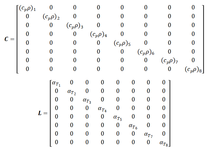
All values of the specific heat diagonal matrix were considered to be , and for the volumetrical expansion a value of was both estimated based on assumptions made by Carvalho (2023).
Source: By the author.
For the heat exchanger coefficient, considering that the reservoir is acting as a heat exchanger, for parametrization purposes it is possible to use the same model AC-M1 from HYDAC mentioned in Carvalho (2023), that uses a cooling specific of approximately 200 W/K.
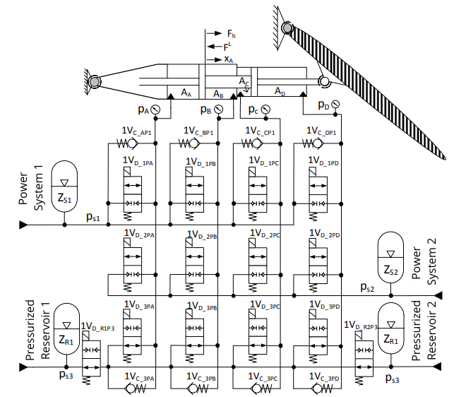
3.5.2. DEHA Thermal Analysis
The DEHA was initially modeled with 17 nodes and 28 corresponding branches. However, considering the cylinder at rest and cruise conditions, analysis can be simplified by using 10 nodes and 15 branches. The reservoir () is connected to three pumps (, , ), each connected to a T-junction (, , ), which in turn are each connected to a relief valve (, , ), a retention (, , ) and a directional valve (, , ). The relief valves lead back to the reservoir and both the retentions and directional valves are connected to an actuator (). The directional valves also lead back to the reservoir, as well as the cylinder.
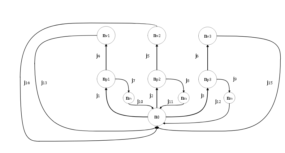
Source: By the author.
The data obtained from Simulink can be seen on Table 8, it was then used to perform the algebraic matricial calculations.
Table 8 – DEHA Simulation Data from Simulink (a) and those used in thermal analysis (b), (c)
| Parameters | Value | Unit |
|---|---|---|
| p₀ | 10 × 10⁵ | Pa |
| P_pump,1 | 1.016 × 10⁶ | Pa |
| P_pump,2 | 1.0072 × 10⁶ | Pa |
| P_pump,3 | 1.0162 × 10⁶ | Pa |
| q_v,pump1 | 2.499 × 10⁻⁵ | m³/s |
| q_v,pump2 | 3.999 × 10⁻⁵ | m³/s |
| q_v,pump3 | 5.998 × 10⁻⁵ | m³/s |
| q_v1,1 | 3.072 × 10⁻⁸ | m³/s |
| q_v2,2 | 5.363 × 10⁻⁸ | m³/s |
| q_v3,3 | 8.828 × 10⁻⁸ | m³/s |
| q_v1,v1 | 2.495 × 10⁻⁵ | m³/s |
| q_v,v2 | 3.995 × 10⁻⁵ | m³/s |
| q_v,v3 | 5.991 × 10⁻⁵ | m³/s |
| p_VP,A | 1.10 × 10⁷ | Pa |
| p_VP,B | 1.10 × 10⁷ | Pa |
| p_VP,C | 1.10 × 10⁷ | Pa |
| p_VP,D | 1.10 × 10⁷ | Pa |
| p_A | 59.03 × 10⁵ | Pa |
| p_B | 11.02 × 10⁵ | Pa |
| p_C | 58.46 × 10⁵ | Pa |
| p_D | 10.45 × 10⁵ | Pa |
| q_v,vPA | -1.014 × 10⁻⁸ | m³/s |
| q_v,vPB | 0 | m³/s |
| q_v,vPC | -5.097 × 10⁻⁸ | m³/s |
| q_v,vPD | 0 | m³/s |
| q_v,vRA | 0 | m³/s |
| q_v,vRB | 8.533 × 10⁻⁹ | m³/s |
| q_v,vRC | 0 | m³/s |
| q_v,vRD | 1.003 × 10⁻⁸ | m³/s |
Source: By the author.
You can download the Project files here: Download files now. (You must be logged in).
For the pressures (b) and flow (c), each branch had a value corresponding to:
| Parameters | Value | Unit |
| P1 | 10 X 10⁵ | Pa |
| P2 | 10 X 10⁵ | Pa |
| P3 | 10 X 10⁵ | Pa |
| P4 | 10.16 X 10⁵ | Pa |
| P5 | 10.072 X 10⁵ | Pa |
| P6 | 10.162 X 10⁵ | Pa |
| P7 | 10.16 X 10⁵ | Pa |
| P8 | 10.072 X 10⁵ | Pa |
| P9 | 10.162 X 10⁵ | Pa |
| P10 | 10 X 10⁵ | Pa |
| P11 | 10 X 10⁵ | Pa |
| P12 | 10 X 10⁵ | Pa |
| P13 | 10 X 10⁵ | Pa |
| P14 | 10 X 10⁵ | Pa |
| P15 | 10 X 10⁵ | Pa |
(c)
| Parameters | Value | Unit |
| qv₁ | 2.498 X 10⁻⁵ | m³/s |
| qv₂ | 4.0 X 10⁻⁵ | m³/s |
| qv3 | 5.999 X 10⁻⁵ | m³/s |
| qv4 | 2.495 X 10⁻⁵ | m³/s |
| qv₅ | 3.995 X 10⁻⁵ | m³/s |
| qv6 | 5.991 X 10⁻⁵ | m³/s |
| qv7 | 3.072 X 10⁻⁸ | m³/s |
| qv₈ | 5.363 X 10⁻⁸ | m³/s |
| qv9 | 8.828 X 10⁻⁸ | m³/s |
| qv₁₀ | 3.072 X 10⁻⁸ | m³/s |
| qv₁₁ | 5.363 X 10⁻⁸ | m³/s |
| qv12 | 8.828 X 10⁻⁸ | m³/s |
| qV13 | 2.495 X 10⁻⁵ | m³/s |
| qv₁₄ | 3.995 X 10⁻⁵ | m³/s |
| 5.991 X 10⁻⁵ | m³/s |
For the DEHA the matrices built are:
Source: By the author.
The same matrices built for the SHA are adapted into the DEHA, those being using the values and assumptions from the tables before, for the SHA.
4. Results and Discussions
4.1. SHA Results
Using the algebraic matricial equations and running the script in MATLAB with all parameters and matrices, the results shown in Table 9 are obtained.
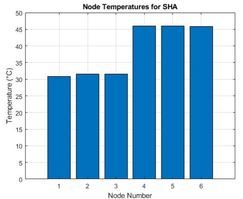
Table 9 – SHA Temperature Results
| Parameters | Value | Unit |
|---|---|---|
| T_reservoir | 30.89 | °C |
| T_pump | 31.53 | °C |
| T_junction | 31.60 | °C |
| T_valve,1 | 45.97 | °C |
| T_valve,2 | 45.97 | °C |
| T_return | 45.90 | °C |
Source: By the author.
Plotting the temperatures from Table 9, it is possible to see the temperature distribution in Figure 22. The reservoir had an increase in temperature of 10.89 , the pump had an increase in temperature of 11.53 , the T-junction an increase and the valves an increase of a little over 15 , with temperatures near 46 . The reservoir, the pump and the T-junction had similar increases in temperature. The fact that the pump had a similar temperature to the reservoir indicates either that it is efficient, or that the energy losses due to pressure drops in the valves are significantly higher.
Source: By the author
4.2. DEHA Results
Similarly to how it was performed in the SHA, considering the proper dimensions and parameters for the DEHA matrices, the results obtained are in Table 10.
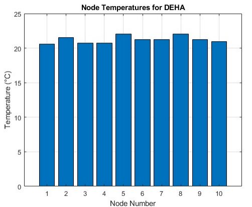
Table 10 – DEHA Temperature Results
| Parameters | Value | Unit |
|---|---|---|
| T_reservoir | 20.62 | °C |
| T_pump,1 | 21.56 | °C |
| T_pump,2 | 20.75 | °C |
| T_pump,3 | 20.77 | °C |
| T_valve,1 | 22.03 | °C |
| T_valve,2 | 22.22 | °C |
| T_valve,3 | 21.24 | °C |
| T_return,1 | 22.03 | °C |
| T_return,2 | 21.22 | °C |
| T_return,3 | 20.97 | °C |
Source: By the author
Plotting the temperatures in MATLAB, a near uniform temperature distribution can be seen across the system, as indicated in Figure 23. In the DEHA, it was observed that all temperatures stayed near the ambient temperature of 20 due to the higher efficiency of the solution. Having more components and significantly smaller pressure drops means there is less energy wasted by throttling and by internal leakage, as leakage depends on pressure and flow.
5. Conclusions
The algebraic mathematical model for temperature prediction of hydraulic systems proved effective in determining the temperatures of each node, obtaining results that approximate temperatures expected from analysis and experiences on similar bench models at LASHIP. While traditional thermal analysis looks at each node individually by comparing the energy entering the node with the energy leaving it, the approach of the algebraic model looks at the system interconnectedly. With the results obtained, it was possible to obtain temperatures at each thermal node using the algebraic mathematical model developed by Carvalho (2023). Comparing the results, it was possible to observe that while the valves of the SHA topology surpassed the temperature of 45 ° C, for the DEHA all components varied little when compared to the room temperature of 20 ° C. Because of this, it is possible to conclude that the DEHA dissipates less energy than the DEHA and is more energetically efficient. This also fits the expected conclusion that the DEHA could work with a smaller heat exchanger than one applied to the SHA. For this bachelor thesis, temperatures were obtained using a simplified equation that does not consider the pipes of the system and their own dissipation. It remains to be determined the effects that pipes could have on heat dissipation and temperature changes,
Additionally, only two topologies were analyzed: SHA and DEHA. To further advance the study of Digital Hydraulics and of the algebraic mathematical model, it is important to apply it in other topologies, such as the DHA and the VSDEHA. Other than this, doing cross analysis with lab experiments and thermal calculations would further test the potential of the algebraic model.
Another limitation is that this analysis was performed to obtain a solution valid on steady-state conditions, which are valid solutions for cruise flights. To obtain a valid solution in transient regimes would be useful for the purposes of evaluating the performance of digital hydraulic systems on more operational conditions.
References
- AKIMOTO, H.; ANODA, Y.; TAKASE, K.; YOSHIDA, T.; TAMAI, H. Nuclear Thermal Hydraulics. Japan: Springer Japan, 2016. 426 p.
- BELAN, C. H. Sistemas de Atuação Hidráulicos Digitais para Aviões com Foco em Eficiência Energética. 2018. 198 p. Tese (Doutorado em Engenharia Mecânica) – Universidade Federal de Santa Catarina, Programa de Pós-Graduação em Engenharia Mecânica – POSMEC, Florianópolis, 2018.
- CARVALHO, L. A. B. Aplicação de Método Algébrico Via Rede Térmica para Predição de Temperatura em Sistemas Hidráulicos. 2023. 126 p. Dissertação (Mestrado em Engenharia Mecânica) – Universidade Federal de Santa Catarina, Programa de Pós-Graduação em Engenharia Mecânica – POSMEC, Florianópolis, 2023.
- CRUZ, D. P. M. Análise de sistemas de atuação hidráulicos digitais para aviões com foco em eficiência energética. 2018. 142 p. Dissertação (Mestrado em Engenharia Mecânica) – Universidade Federal de Santa Catarina, Programa de Pós-Graduação em Engenharia Mecânica – POSMEC, Florianópolis, 2018.
- DELL’AMICO, A.; CARLSSON, M.; NORLIN, E.; SETHSON, M. Investigation of a Digital Hydraulic Actuation System on an Excavator Arm. In: 13th Scandinavian International Conference on Fluid Power – SICFP, Linköping, Sweden, 2013.
- DURFEE, W. A.; ZONGXUAN, S.; VAN DE VEN, J. D. Fluid Power System Dynamics. Department of Mechanical Engineering, University of Minnesota, 2015. 54 p.
- DZOMENE, F. A. J. Design of a linear actuated Electrohydraulic servo valve for tree shaker applications with the hydraulic test bench. 66 p. Dissertação (Mestrado em Engenharia Mecânica) – Department of Mechanical and Aerospace Engineering, Politecnico di Torino & Université de Technologie de Compiègne, 2021.
- FEDERAL AVIATION ADMINISTRATION (FAA). Pilot’s Handbook of Aeronautical Knowledge. 2016th ed. Newcastle, WA, USA: Aviation Supplies & Academics, 2016. 524 p.
- LINJAMA, M. Digital Fluid Power – State of the Art. In: Proceedings of the 12th Scandinavian International Fluid Power Conference, v. 3, p. 331, 2011.
- LINJAMA, M. Energy Saving Digital Hydraulics. In: Second Workshop on Digital Fluid Power, Linz, Austria, 2009.
- LOPES JUNIOR, R. S. Avaliação do desempenho dinâmico de um atuador hidráulico digital para aplicações aeronáuticas em condição de falha. 2021. 153 p. Dissertação (Mestrado em Engenharia Mecânica) – Universidade Federal de Santa Catarina, Programa de Pós-Graduação em Engenharia Mecânica – POSMEC, Florianópolis, 2021.
- MANTOVANI, J. I. Otimização dos Chaveamentos entre Válvulas on/off em Atuadores Hidráulicos Digitais. 2019. 140 p. Dissertação (Mestrado em Engenharia Mecânica) – Universidade Federal de Santa Catarina, 2019.
- NOSTRANI, M. P. Development Of A Digital Electro Hydrostatic Actuator For Application In Aircraft Flight Control Surfaces. 192 p. Tese (Doutorado) – Universidade Federal de Santa Catarina, Programa de Pós-Graduação em Engenharia Mecânica – POSMEC, Florianópolis, 2021.
- OXFORD ECONOMICS. Economic Benefits from Air Transport in the UK. UK Country Report, 2011. Disponível em: http://www.niassembly.gov.uk/globalassets/documents/finance-2011-2016/air-passenger-duty/written-submissions/oxford-economics-economic-benefitsfrom-air-transport-in-uk.pdf. Acesso em: 18 abr. 2023.
- PINTARELLI, M. B. Modeling and parametric identification of an EHSA considering thermal effects on damped mode. 92 p. Dissertação (Mestrado em Engenharia Mecânica e Aeronáutica) – Instituto Tecnológico de Aeronáutica, São José dos Campos, 2022.
- RONGJIE, K.; ZONGXIA, J.; SHAOPING, W.; LISHA, C. Design and Simulation of Electrohydrostatic Actuator with a Built-in Power Regulator. Chinese Journal of Aeronautics, v. 22, n. 6, p. 700–706, 2009.
- SADRAEY, M. H. Aircraft Design: A Systems Engineering Approach. Chichester, West Sussex, U.K.: Wiley, 2013. 800 p.
- Válvula direcional – Fig 7. Disponível em: https://www.unilim.fr/pages_perso/thierry.cortier/Hydraulique_cours/co/Hydraulique_-_De_la_mecanique_des_fluides_a_la_transmission_de_Puissance.html. Acesso em: 14 jul. 2025.
- SILVA, D. O. Variable speed digital electro-hydraulic actuator for aircraft application. 212 p. Tese (Doutorado) – Universidade Federal de Santa Catarina, Programa de Pós-Graduação em Engenharia Mecânica – POSMEC, Florianópolis, 2023.
You can download the Project files here: Download files now. (You must be logged in).


Responses