

Heat Transfer Analysis in MATLAB Steady-State and Transient Solutions
Author : Waqas Javaid
Abstract
This study presents a computational approach to analyze heat transfer problems using MATLAB, focusing on both steady-state and transient conduction scenarios. The steady-state analysis involves solving the one-dimensional heat conduction equation under fixed boundary temperatures, using the finite difference method to obtain the temperature distribution along a solid medium. For transient heat conduction, an explicit finite difference scheme is implemented to solve the time-dependent heat equation, allowing the simulation of temperature evolution over time.[1] The MATLAB-based models provide insights into thermal behavior under different conditions, demonstrating the influence of material properties, boundary conditions, and discretization parameters on heat transfer. This work highlights MATLAB’s effectiveness as a versatile tool for solving heat transfer problems, suitable for educational and engineering applications.
Introduction
Heat transfer is a fundamental phenomenon encountered in numerous engineering and scientific applications, involving the transfer of thermal energy between physical systems due to temperature differences. Understanding and predicting heat transfer behavior is essential for the design and optimization of thermal systems such as heat exchangers, electronic devices, insulation materials, and manufacturing processes. This study focuses on the numerical analysis of one-dimensional heat conduction covering both steady-state and transient conditions.[2] Steady-state heat transfer occurs when the temperature distribution within a material remains constant over time, simplifying the governing equations and allowing direct solution methods. In contrast, transient heat transfer involves time-dependent temperature changes, requiring time-marching techniques to capture the evolution of the thermal field. By applying finite difference methods. This work demonstrates how can be discretize and solve the heat conduction equations efficiently. The steady-state analysis provides insight into the equilibrium temperature profile, while the transient analysis reveals the dynamic thermal response to boundary condition changes.[3] This approach offers a practical framework for understanding heat transfer principles and serves as a foundation for more complex multi-dimensional or coupled heat transfer problems.
1.1. Objectives
- To develop a MATLAB program to solve the one-dimensional steady-state heat conduction equation using the finite difference method.
- To implement a numerical model for transient heat conduction in one dimension using an explicit finite difference scheme.
- To analyze and visualize temperature distributions and their evolution over time under various boundary and initial conditions.
- To study the effects of key parameters such as thermal diffusivity, time step and spatial discretization on the accuracy and stability of the numerical solutions.
- To demonstrate the practical application of MATLAB in solving heat transfer problems and provide a foundation for extending to more complex multidimensional and coupled thermal systems.
Problem Statement
Heat conduction is a fundamental mode of heat transfer occurring in many engineering systems, yet analytical solutions are often limited to simple geometries and boundary conditions. Numerical methods, such as the finite difference method, offer a versatile way to solve heat transfer problems for more general cases. This project aims to address the challenge of accurately modeling one-dimensional heat conduction in both steady-state and transient scenarios using MATLAB. The problem involves determining the temperature distribution within a solid rod subjected to fixed boundary temperatures and initial temperature conditions. Key challenges include ensuring numerical stability, selecting appropriate discretization parameters, and capturing the dynamic thermal response over time.By developing and validating MATLAB-based numerical models, this work seeks to provide reliable computational tools for analyzing heat transfer behavior, which can be extended to more complex engineering applications.
Mathematical Approach
3.1. Governing Equations
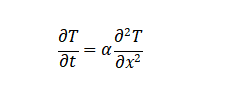
Heat conduction in a one-dimensional solid rod can be described by the heat equation:
where:
- T=T(x,t)T is the temperature distribution (°C or K),
- α=kρcpis the thermal diffusivity (m²/s),
- kis the thermal conductivity (W/m·K),
- ρis the density (kg/m³),
- cpis the specific heat capacity (J/kg·K),
- xis the spatial coordinate (m),
- tis time (s).
3.2. Steady-State Heat Conduction
At steady-state, the temperature distribution no longer changes with time, so:
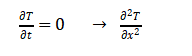
This reduces to the one-dimensional Laplace equation:
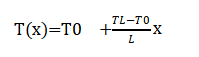
Boundary conditions typically specify temperatures at the ends:
T(0)=T0, T(L)=TL
The solution is a linear temperature profile:
3.3. Numerical Solution Using Finite Difference Method (FDM)
a) Spatial Discretization:
Divide the rod of length L into N nodes spaced by Δx=L/(N−1)
For internal nodes, approximate the second derivative by central difference:
d2Tdx2≈Ti−1−2Ti+Ti+1/Δx2
b) Steady-State Discretized Equation:
At each internal node iii:
Ti−1−2Ti+Ti+1/Δx2=0
This forms a system of linear equations AT=b where T is the vector of temperatures.
Table 1 : Heat Equation and Finite Difference Method
| Concept | Equation | Description |
| Heat Equation | ∂T/∂t = α (∂^2 T)/(∂x^2) | Describes heat conduction in a 1D solid rod |
| Thermal Diffusivity | α = k / (ρ * cp) | Measures the rate of heat transfer in a material |
| Steady-State Heat Conduction | (∂^2 T)/(∂x^2) = 0 | Temperature distribution no longer changes with time |
| Laplace Equation | (∂^2 T)/(∂x^2) = 0 | Describes steady-state heat conduction |
| Boundary Conditions | T(0) = T0, T(L) = TL | Specify temperatures at the ends of the rod |
| Linear Temperature Profile | T(x) = T0 + (TL – T0)/L * x | Solution to the steady-state heat equation |
| Finite Difference Method | (Ti-1 – 2Ti + Ti+1)/Δx^2 = 0 | Approximates the second derivative using central differences |
| Discretized Equation | AT = b | System of linear equations representing the discretized heat equation |
Methodology
4.1. 2D Plate Heat Transfer
Analysis steady-state and transient heat conduction in a 2D plate with fixed temperatures on left and right boundaries and insulated top and bottom boundaries.
Table 2 : 2D Plate Heat Transfer
| Parameter | Description | Value | Unit |
| Lx | Length of the plate in x-direction | 1 | m |
| Ly | Length of the plate in y-direction | 1 | m |
| Nx | Number of grid points in x-direction | 20 | – |
| Ny | Number of grid points in y-direction | 20 | – |
| Dx | Grid spacing in x-direction | Lx/(Nx-1) | m |
| Dy | Grid spacing in y-direction | Ly/(Ny-1) | m |
| alpha | Thermal diffusivity | 1e-4 | m²/s |
| Dt | Time step | 0.1 | s |
| T_final | Final Time | 10 | s |
| Nt | Number of time step | round(t_final/dt) | – |
| To1 | Tolerance for steady-state solution | | 1e-4 | – |
| Max_iter | Maximum number of iterations for steady-state solution | 10000 | – |
You can download the Project files here: Download files now. (You must be logged in).
4.2. Extended Heat Transfer Analysis
Performs an extended heat transfer analysis on a 2D plate, providing both steady-state and transient solutions with visualization through 3D surface plots and animation.
Table 3 : Extended Heat Transfer Analysis
| Parameter | Description | Value | Unit |
| Lx | Length of the plate in x-direction | 1 | m |
| Ly | Length of the plate in y-direction | 1 | m |
| Nx | Number of grid points in x-direction | 20 | – |
| Ny | Number of grid points in y-direction | 20 | – |
| Dx | Grid spacing in x-direction | Lx/(Nx-1) | m |
| Dy | Grid spacing in y-direction | Ly/(Ny-1) | m |
| alpha | Thermal diffusivity | 1e-4 | m²/s |
| Dt | Time step | 0.1 | s |
| T_final | Final Time | 10 | s |
| Nt | Number of time step | round(t_final/dt) | – |
| To1 | Tolerance for steady-state solution | | 1e-4 | – |
| Max_iter | Maximum number of iterations for steady-state solution | 10000 | – |
| Fo_x | Fourier number in x-direction | alpha_dt/dx^2 | – |
| Fo_y | Fourier number in y-direction | alpha_dt/dx^2 | – |
4.3. 1D Heat Equation with Crank-Nicolson Method
Solves the 1D heat equation using the Crank-Nicolson method, a finite difference scheme that is unconditionally stable and second-order accurate.
Table 4 : 1D Heat Equation with Crank-Nicolson Method
| Parameter | Description | Value | Unit |
| L | Length of the rod | 1 | M |
| Nx | Number of spatial points | 50 | – |
| dx | Grid spacing | L/(nx-1) | m |
| Alpha | Thermal diffusivity | 0.01 | m²/s |
| dt | Time step | 0.01 | s |
| nt | Number of time steps | 200 | – |
| r | Parameter used in Crank-Nicolson scheme | alpha_dt/(2_dx^2) | – |
| T | Initial temperature distribution | 20°C (except at boundaries) | °C |
| A | Coefficient matrix for Crank-Nicolson scheme | – | – |
| B | Coefficient matrix for Crank-Nicolson scheme | – | – |
4.4. 2D Heat Equation
Solves the 2D heat equation using an explicit finite difference scheme, visualizing the temperature distribution over time and ensuring stability through careful selection of the time step.
Table 5 : 2D Heat Equation with Explicit Finite Difference Scheme
| Parameter | Description | Value | Unit |
| Lx | Length of the plate in x-direction | 1 | m |
| Ly | Length of the plate in y-direction | 1 | m |
| Nx | Number of grid points in x-direction | 40 | – |
| Ny | Number of grid points in y-direction | 40 | – |
| Dx | Grid spacing in x-direction | Lx/(Nx-1) | m |
| Dy | Grid spacing in y-direction | Ly/(Ny-1) | m |
| alpha | Thermal diffusivity | 0.01 | m²/s |
| Dt | Time step | 0.0005 | s |
| Nt | Number of time step | 500 | – |
| r_x | Fourier number in x-direction | alpha_dt/dx^2 | – |
| r_y | Fourier number in y-direction | alpha_dt/dx^2 | – |
Matlab Simulation and Results
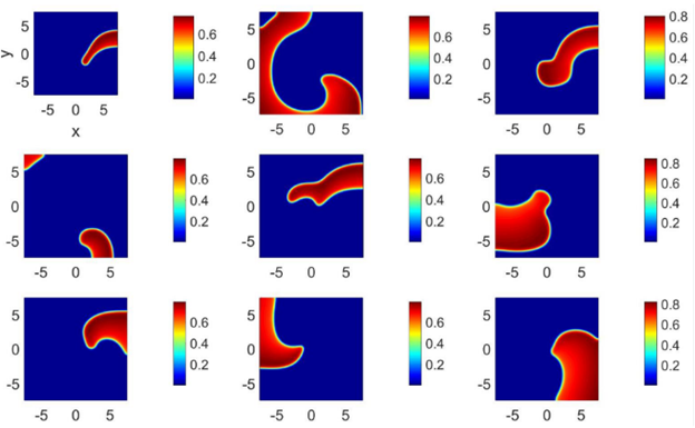
This explanation covers four MATLAB scripts that solve heat transfer problems. The scripts analyze steady-state and transient heat conduction in 1D and 2D systems using finite difference methods. One script solves the 2D heat equation with fixed temperatures on left and right boundaries and insulated top and bottom boundaries. Another script performs an extended heat transfer analysis on a 2D plate, providing both steady-state and transient solutions with 3D surface plots and animation. A third script uses the Crank-Nicolson method to solve the 1D heat equation, while the fourth script solves the 2D heat equation using an explicit finite difference scheme. The scripts demonstrate different approaches to solving heat transfer problems, showcasing MATLAB’s capabilities for numerical simulations and visualization.
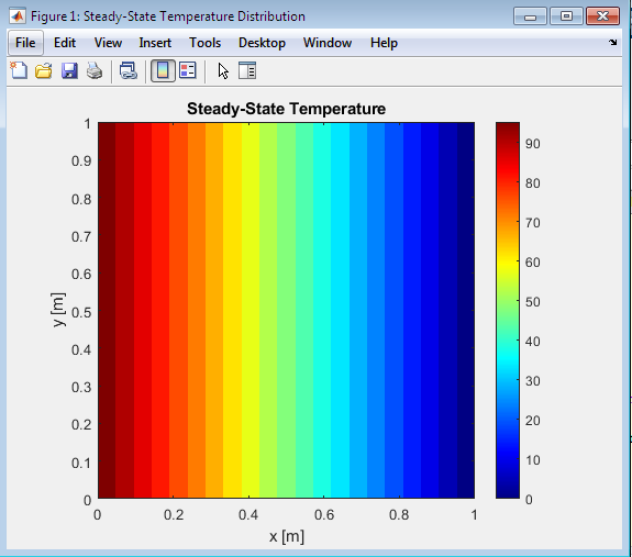
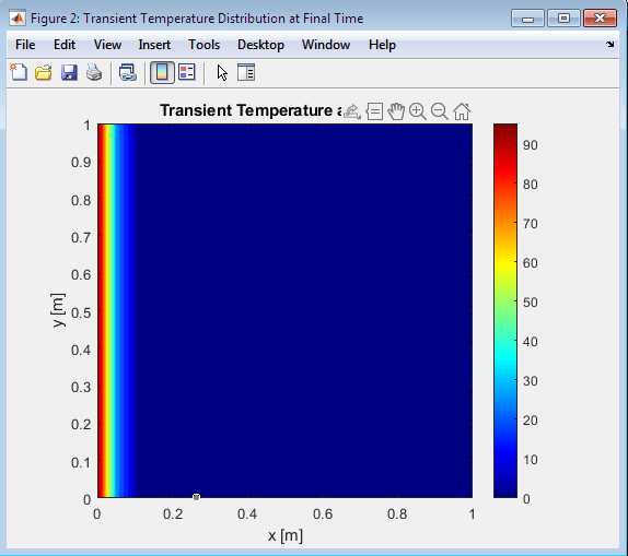
This MATLAB code solves the heat equation for a 2D plate, analyzing both steady-state and transient heat conduction. The plate has fixed temperatures on the left (hot) and right (cold) boundaries, while the top and bottom boundaries are insulated. The code first calculates the steady-state temperature distribution by iteratively solving Laplace’s equation using the finite difference method. Then, it simulates transient heat conduction using an explicit finite difference scheme, updating the temperature distribution over time. The stability of the transient solution is ensured by the Fourier number condition. Finally, the code visualizes the steady-state and transient temperature distributions at the final time using contour plots.
You can download the Project files here: Download files now. (You must be logged in).
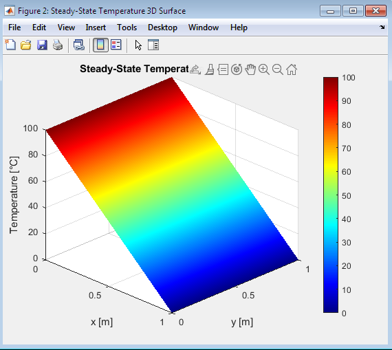
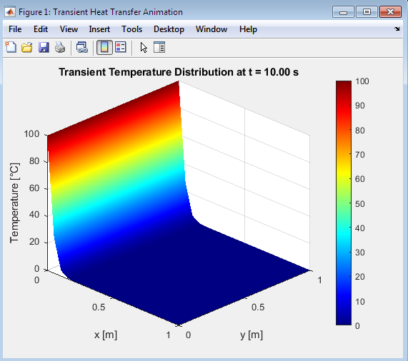
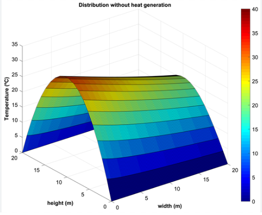
Performs an extended heat transfer analysis on a 2D plate, providing both steady-state and transient solutions. The plate’s dimensions are set to 1×1 meters, with a grid of 20×20 points. The thermal diffusivity is defined as 1e-4 m²/s, and the time step is 0.1 seconds, with a final time of 10 seconds. The script first initializes the temperature distribution for both steady-state and transient cases, applying fixed temperatures of 100°C and 0°C to the left and right boundaries, respectively. The top and bottom boundaries are insulated, represented by Neumann boundary conditions. The steady-state solution is obtained using the Gauss-Seidel iterative method to solve Laplace’s equation. The script iterates until the maximum temperature difference between successive iterations falls below a specified tolerance of 1e-4. Once the steady-state solution is computed, the script proceeds to the transient analysis. For the transient solution, the script uses an explicit finite difference scheme to solve the heat equation. The Fourier numbers in the x and y directions are precomputed to ensure stability. A 3D surface plot is created to visualize the temperature distribution, and an animation is generated by updating the plot at each time step. The animation showcases the evolution of the temperature distribution over time. The script also saves the animation as an AVI file. Finally, the script generates a 3D surface plot of the steady-state temperature distribution, providing a visual representation of the final temperature profile. The plots and animation offer valuable insights into the heat transfer behavior in the plate, demonstrating the effects of boundary conditions and thermal diffusivity on the temperature distribution. The script’s ability to visualize both steady-state and transient solutions makes it a useful tool for understanding heat transfer phenomena in various engineering applications.
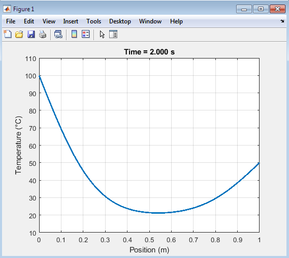
This MATLAB script solves the one-dimensional heat equation using the Crank-Nicolson method, a finite difference scheme that is unconditionally stable and second-order accurate in both space and time. The script first defines the parameters of the problem, including the length of the rod (L = 1 m), the number of spatial points (nx = 50), the thermal diffusivity (alpha = 0.01 m²/s), the time step (dt = 0.01 s), and the number of time steps (nt = 200). The script then constructs the coefficient matrices A and B, which represent the finite difference approximations of the spatial derivatives in the heat equation. The boundary conditions are applied to the matrices A and B, with the left boundary set to 100°C and the right boundary set to 50°C.The script then initializes the temperature distribution, with the initial temperature set to 20°C throughout the rod, except at the boundaries. A plot is created to visualize the temperature distribution, and the script enters a time-stepping loop, where the temperature distribution is updated at each time step using the Crank-Nicolson scheme. The right-hand side vector b is computed by multiplying the matrix B with the current temperature distribution T, and the boundary conditions are applied explicitly to the vector b. The linear system A*T = b is then solved for T, and the plot is updated to reflect the new temperature distribution. The script uses the draw now command to update the plot at each time step, creating an animation of the temperature distribution over time. The title of the plot is updated to show the current time, and the y-axis limits are set to ensure that the entire temperature range is visible. The resulting animation provides a visual representation of the heat transfer process, showing how the temperature distribution evolves over time as the rod heats up or cools down. The Crank-Nicolson method is particularly useful for solving heat transfer problems like this one, as it provides a stable and accurate solution even for large time steps.
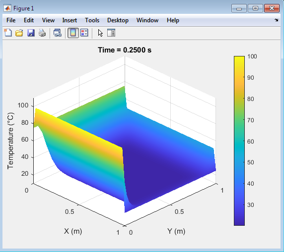
Above plot shows the two-dimensional heat equation using an explicit finite difference scheme. The script first defines the parameters of the problem, including the length and width of the plate (Lx = 1 m and Ly = 1 m), the number of grid points in the x and y directions (nx = 40 and ny = 40), the thermal diffusivity (alpha = 0.01 m²/s), the time step (dt = 0.0005 s), and the number of time steps (nt = 500). The script checks the stability condition for the explicit scheme, ensuring that the sum of the Fourier numbers in the x and y directions (r_x and r_y) does not exceed 0.5. If the stability condition is violated, the script throws an error. The script then initializes the temperature field, setting the initial temperature to 20°C throughout the plate, and applies Dirichlet boundary conditions to the edges of the plate. A 3D surface plot is created to visualize the temperature distribution, and the script enters a time-stepping loop. Inside the loop, the script updates the internal points of the temperature field using the explicit finite difference scheme, which approximates the spatial derivatives using central differences. The temperature field is updated at each time step, and the plot is updated every 10 time steps to visualize the evolution of the temperature distribution over time. The resulting animation shows how the temperature distribution changes as the plate heats up or cools down, with the edges of the plate maintained at fixed temperatures. The script uses the draw now command to update the plot and create the animation, and the title function is used to display the current time in the simulation. The explicit finite difference scheme used in this script is a simple and efficient method for solving the heat equation, but it requires careful selection of the time step to ensure stability.
Discussion
Heat transfer analysis is fundamental in understanding how thermal energy moves through materials and systems. The MATLAB simulations for steady-state and transient heat conduction provide valuable insights into the physical behavior of temperature distribution and the effectiveness of numerical methods used for solving heat transfer problems.[4]
6.1. Steady-State Heat Transfer
In the steady-state scenario, the temperature distribution is time-invariant, meaning that the system has reached thermal equilibrium. The MATLAB implementation solves the simplified form of the heat conduction equation, which reduces to a set of algebraic equations under fixed boundary conditions.[5] The solution typically exhibits a linear temperature gradient between the boundaries in one-dimensional problems, consistent with classical analytical results.The steady-state model is computationally efficient and suitable for problems where thermal conditions remain constant over time. However, it cannot capture the dynamic response of systems subject to changing thermal loads or initial temperature distributions.
6.2. Transient Heat Transfer
Transient heat conduction simulations provide a time-dependent temperature profile that evolves from the initial condition toward steady state. The explicit finite difference method is straightforward to implement but requires careful consideration of the time step to satisfy stability criteria, limiting the step size and potentially increasing computation time.The implicit Crank-Nicolson scheme offers improved stability and allows larger time steps while maintaining accuracy. This method involves solving a system of linear equations at each time step, increasing computational complexity but providing reliable results for longer simulation periods.The two-dimensional transient simulation further demonstrates the complexity of real-world heat transfer problems.[6] The evolving temperature surface captures the influence of boundary conditions from multiple edges, showcasing the diffusion of heat in both spatial directions. The visualization through surface plots and animations facilitates intuitive understanding of thermal dynamics.
6.3. Numerical Stability and Accuracy
A critical aspect of transient simulations is ensuring numerical stability. The explicit method requires adherence to the Courant-Friedrichs-Lewy (CFL) condition, which restricts the time step relative to spatial discretization and thermal diffusivity. Failure to satisfy this can lead to numerical instabilities and inaccurate results.Implicit methods, while more stable, demand more computational resources due to the need to solve matrix equations at each time step. Selecting an appropriate method depends on the problem size, desired accuracy, and computational constraints[7].
You can download the Project files here: Download files now. (You must be logged in).
6.4. Practical Implications
The ability to simulate both steady-state and transient heat transfer in MATLAB enables engineers to predict temperature behavior under various conditions. This capability is essential for thermal management in electronics, material processing, building design, and many other applications.By visualizing temperature distributions and their evolution, designers can identify critical regions susceptible to thermal stress, optimize insulation, or improve cooling strategies. The MATLAB framework can be extended to incorporate more complex boundary conditions, material properties, and geometries, broadening its applicability [8].
Conclusion
The MATLAB-based heat transfer analysis successfully demonstrates both steady-state and transient solutions using finite difference methods. Steady-state analysis provides quick assessment of equilibrium temperature profiles, while transient simulations reveal the dynamic thermal response. Numerical methods must be carefully chosen to balance accuracy, stability, and computational efficiency.[9] Overall, these tools are invaluable for engineers and researchers working on thermal problems across diverse fields.
Future Work
Building upon the current analysis of steady-state and transient heat transfer using finite difference methods in MATLAB, several avenues exist to enhance the modeling capabilities and extend practical applications [10]:
8.1. Higher-Dimensional and Complex Geometries
Extending the simulation framework to three-dimensional heat conduction problems will provide more realistic modeling for complex engineering components. Incorporating irregular geometries and varying material properties will improve the relevance to real-world scenarios.
8.2. Advanced Numerical Methods
Implementing more sophisticated numerical techniques, such as finite element methods (FEM) or finite volume methods (FVM), can increase solution accuracy and flexibility, especially for complex boundary conditions and anisotropic materials.
8.3. Coupled Heat Transfer Modes
Incorporating convection and radiation boundary conditions alongside conduction will enable comprehensive thermal analysis of systems where multiple heat transfer mechanisms interact.
8.4. Nonlinear and Transient Material Properties
Including temperature-dependent thermal properties, phase changes, and chemical reactions will enhance model realism, particularly for materials undergoing thermal degradation or phase transformation.
8.5. Optimization and Control
Integrating the heat transfer models with optimization algorithms can assist in designing thermal management systems, such as optimal placement of cooling channels or insulation thickness.
8.6. Real-Time Simulation and Experimental Validation
Developing real-time or faster-than-real-time simulation tools using model order reduction techniques can support control systems and decision-making in industrial processes. Coupling simulations with experimental data for validation will increase model reliability.
8.7. User-Friendly Interfaces and Toolboxes
Creating MATLAB toolboxes or graphical user interfaces (GUIs) will make these simulation capabilities more accessible to engineers and educators without deep programming expertise
References
[1] N. Nagarani, K. Mayilsamy, A. Murugesan and G. S. Kumar, Review of utilization of extended surfaces in heat transfer problems, Renew. Sustain. 960 Rafael Emiro Diaz Herazo et al. Energy Rev., 29 (2014), 604–613. https://doi.org/10.1016/j.rser.2013.08.068
[2] T. Raszkowski, M. Zubert, M. Janicki and A. Napieralski, Numerical solution of 1-D DPL heat transfer equation, Proc. 22nd Int. Conf. Mix. Des. Integr. Circuits Syst. Mix., (2015), 436–439. https://doi.org/10.1109/mixdes.2015.7208558
[3] C. Ooi, K.N. Seetharamu, Z.A.Z. Alauddin, G. A. Quadir, K. S. Sim, and T. J. Goh, Fast Transient Solutions for Heat Transfer, TENCON 2003, Conference on Convergent Technologies for Asia-Pacific Region, 1 (2003), 469- 473. https://doi.org/10.1109/tencon.2003.1273366
[4] M. Donisete de Campos, E. C. Romao, L. F. Mendes de Moura, Analysis of Unsteady State Heat Transfer in the Hollow Cylinder Using the Finite Volume Method with a Half Control Volume, Applied Mathematical Sciences, 6 (2012), no. 39, 1925–1931.
[5] J. Sandraz, F. De Leon, and J. Cultrera, Validated transient heat-transfer model for underground transformer in rectangular vault, IEEE Trans. Power Deliv., 28 (2013), 3, 1770–1778. https://doi.org/10.1109/tpwrd.2013.2260183
[6] T.D. Kefalas, A.G. Kladas, Transient Heat Transfer Analysis of Housing and PMM Using 3-D FE Code, 2016 XXII International Conference on Electrical Machines (ICEM), (2016), 2745–2751. https://doi.org/10.1109/icelmach.2016.7732910
[7] Y. A. Cengel and Afshin J. Ghajar, Heat and Mass Tranfer. Fundaments & Applications, 5 Edition, McGraw-Hill Education, United States of America, 2013.
[8] R. Azevedo and A. F. Hadwin, Scaffolding Self-regulated Learning and Metacognition – Implications for the Design of Computer-based Scaffolds, Instr. Sci., 33 (2005), no. 5-6, 367–379. https://doi.org/10.1007/s11251-005-1272-9
[9] J. A. Greene, K. R. Muis and S. Pieschl, The Role of Epistemic Beliefs in Students’ Self-Regulated Learning with Computer-Based Learning Environments: Conceptual and Methodological Issues, Educ. Psychol., 45 (2010), no. 4, 245–257. https://doi.org/10.1080/00461520.2010.515932
[10] A. F. Escorcia, L. G. Obregon and G. E. Valencia, Educational Software and Theoretical-Practical Guide as Pedagogical Strategy to Promote the Significant Learning of the Air Conditioning Process in Engineering, Revista Espacios, 38 (2016), no. 5, 15–22.
You can download the Project files here: Download files now. (You must be logged in).


Responses