

Fractals and Chaos: A MATLAB-Based Exploration of the Mandelbrot Set and Logistic Map Dynamics
Author : Waqas Javaid
Abstract
This article presents a comprehensive mathematical and computational exploration of fractal geometry and chaotic behavior using MATLAB. The study focuses on two fundamental nonlinear systems: the Mandelbrot set and the logistic map, both of which exhibit complex dynamics arising from simple iterative rules. The concept of fractals was first popularized by Benoit B. Mandelbrot, who demonstrated that complex geometric structures can emerge from simple iterative rules [1]. The Mandelbrot set is generated through the quadratic recurrence relation , visualized using escape-time coloring to reveal its intricate self-similar structure and fractal boundaries. The logistic map is investigated to demonstrate transitions from stability to chaos as the control parameter varies. The Logistic Map is one of the simplest mathematical models exhibiting chaotic behavior, illustrating how nonlinearity leads to unpredictable outcomes even in deterministic systems [2]. MATLAB simulations produce the bifurcation diagram, illustrating the period-doubling route to chaos, and compute the Lyapunov exponent, which quantitatively distinguishes regular and chaotic regions. MATLAB provides an efficient computational environment for iterating complex equations and visualizing the resulting fractal and chaotic structures with high precision [3]. Through numerical iteration, data visualization, and parameter analysis, the project highlights the deep interconnection between deterministic rules and unpredictable outcomes. The results confirm that even simple nonlinear equations can produce infinitely complex behavior, offering valuable insights into nonlinear dynamics, stability analysis, and fractal mathematics. The comparison between the Mandelbrot Set and Logistic Map reveals that both share common features of sensitivity to initial conditions and parameter dependence, which are hallmarks of chaotic systems [4]. This study demonstrates MATLAB’s capability as a powerful tool for modeling, visualizing, and understanding the fascinating world of chaos and fractals.
Introduction
The study of nonlinear systems, chaos theory, and fractal geometry has emerged as one of the most fascinating areas of applied mathematics and computational science. Unlike traditional linear models, nonlinear dynamical systems can exhibit highly complex and unpredictable behavior, even when governed by simple deterministic equations. Previous studies have shown that iterative complex mappings generate visually rich fractal structures with self-similarity across scales [5].This apparent paradox order hidden within apparent random nessforms the core of chaos theory. Among the mathematical models that illustrate this phenomenon, the Mandelbrot set and the logistic map stand as iconic examples.
The Mandelbrot set, discovered by Benoît Mandelbrot in the late twentieth century, is a collection of complex numbers that produces an infinitely detailed boundary exhibiting self-similarity and intricate fractal patterns. The boundary points of the Mandelbrot set provide valuable insight into the stability of complex dynamical systems [6].It symbolizes the geometric beauty of mathematical recursion and serves as a visual gateway to understanding fractal geometry. On the other hand, the logistic map, introduced by Robert May, models population growth under nonlinear feedback and provides a simple yet profound example of how deterministic systems can evolve into chaotic regimes as a parameter changes. Chaotic regimes in the Logistic Map are often analyzed using bifurcation diagrams to reveal transitions from order to chaos [7].The motivation for this study lies in exploring how MATLAB, a high-level numerical computing environment, can be employed to simulate, visualize, and analyze such nonlinear phenomena with both mathematical rigor and graphical precision. MATLAB’s matrix-based computation, powerful plotting tools, and iterative programming capabilities make it an ideal platform for studying complex systems. This project aims to simulate the generation of the Mandelbrot set through iterative complex mappings and to analyze the dynamic behavior of the logistic map by constructing bifurcation diagrams and evaluating Lyapunov exponents. Computational visualization of fractals helps in understanding nonlinear behaviors that are otherwise analytically intractable [8]. These simulations not only demonstrate the theoretical concepts of chaos and fractal structure but also provide a visual understanding of stability, periodicity, and sensitivity to initial conditions.
By bridging mathematical theory with computational implementation, this work offers deeper insight into how simple mathematical rules can produce infinite complexity, highlighting the universal presence of chaos and fractal patterns in nature, physics, and engineering systems.
1.1. Background and Motivation
In mathematics and physics, many real-world systems are inherently nonlinear, meaning their output does not change proportionally with their input. Such systems often display complex, unpredictable, and sensitive behavior, which cannot be explained using classical linear models. The emergence of chaos theory in the twentieth century provided a framework to study these unpredictable yet deterministic systems. Chaos theory reveals that even simple equations can produce irregular and highly intricate patterns over time. This unpredictable nature of deterministic systems has led to a growing interest in exploring their mathematical structure and behavior. The color-coded representation of the Mandelbrot Set enhances the distinction between convergent and divergent regions [9].
1.2. Fractals and Their Significance
One of the most remarkable discoveries in nonlinear mathematics is the concept of fractals geometrical shapes that exhibit self-similarity at different scales. A fractal repeats its pattern infinitely, regardless of the level of magnification. The Mandelbrot set, named after Benoît Mandelbrot, is one of the most famous examples of such a structure. Increasing the number of iterations in the algorithm produces more detailed and accurate fractal boundaries [10]. It is generated from a simple iterative equation involving complex numbers, yet it produces visually stunning patterns of infinite detail and complexity. Fractals are not just mathematical curiosities; they are found in nature in coastlines, clouds, plants, and biological structures showing how mathematical recursion can model natural growth and irregularity.
1.3. Chaos and Nonlinear Dynamics
While fractals describe spatial self-similarity, chaos theory explains the temporal unpredictability of dynamic systems. A classical example is the logistic map, an equation that models population growth under constrained environmental conditions. The MATLAB simulation enables efficient control over parameters such as iteration count, scaling, and complex plane limits [11].As the control parameter changes, the logistic map transitions from stable equilibrium to periodic oscillations and eventually to chaotic behavior. This transition, known as the period-doubling route to chaos, illustrates how order gradually gives way to disorder in deterministic systems. The bifurcation diagram of the logistic map visually demonstrates these transitions, while the Lyapunov exponent quantifies the degree of sensitivity to initial conditions a hallmark of chaos.
1.4. Role of MATLAB in the Study
To explore these fascinating phenomena, MATLAB serves as an ideal computational platform. It combines mathematical accuracy with advanced visualization tools, enabling detailed numerical experimentation and graphical representation. MATLAB’s capability for handling iterative computations and complex arithmetic allows researchers to simulate fractal structures such as the Mandelbrot set and to analyze the dynamics of chaotic systems like the logistic map. A zoom-in process on specific regions of the Mandelbrot Set reveals infinite complexity and self-repeating patterns [12].Through scripting and plotting, MATLAB helps bridge theoretical mathematics with practical simulation, offering both insight and intuition into nonlinear behavior.
1.5. Objectives
The main objectives of this project are:
- To generate and visualize the Mandelbrot set using iterative complex mappings.
- To investigate the logistic map for various parameter values and observe its dynamic behavior.
- To construct the bifurcation diagram showing the transition from stability to chaos.
- To compute and analyze the Lyapunov exponent to distinguish between periodic and chaotic regimes.
1.6. Importance and Relevance
The study of fractals and chaos is not merely theoretical; it has wide-ranging applications in engineering, physics, biology, finance, and computer graphics. Understanding chaotic systems improves modeling in weather prediction, secure communication, and control system design. Similarly, fractal geometry aids in data compression, pattern recognition, and natural image modeling. The Logistic Map provides a powerful framework for studying population dynamics and ecological growth patterns [13]. By using MATLAB to explore these mathematical ideas, this project provides a hands-on understanding of how computational tools can reveal the underlying order in seemingly random behavior. The presence of chaos is confirmed by sensitive dependence on initial conditions and nonlinear feedback mechanisms [14].
Problem Statement
The study of nonlinear dynamical systems presents a major challenge in understanding how simple mathematical equations can produce highly complex and unpredictable behavior. Traditional analytical methods are often insufficient to capture the intricate patterns and transitions observed in such systems. This project addresses the problem of visualizing and analyzing chaotic and fractal phenomena using computational techniques. Specifically, it investigates how the Mandelbrot set reveals fractal geometry through iterative complex mappings, and how the logistic map exhibits the transition from stability to chaos as its control parameter varies. By using MATLAB to simulate, visualize and analysis these models, the project aims to illustrate the underlying mathematical mechanisms that govern fractal formation and chaotic dynamics in nonlinear systems.
Mathematical Approach
The mathematical foundation of this article is based on iterative equations that describe nonlinear behavior in both complex and real domains. Two primary mathematical models are employed: the Mandelbrot set and the logistic map, each illustrating a different aspect of chaos and fractal geometry.
3.1. Mandelbrot Set
The Mandelbrot set is defined by the iterative complex quadratic function:
z_{n+1} = z_n^2 + c
A complex number belongs to the Mandelbrot set if the sequence remains bounded as . In practical computation, the iteration is performed up to a maximum number of steps , and the point is considered part of the set if for all. The escape-time algorithm is used to visualize the set: each pixel in the complex plane represents a value of , and its color corresponds to the number of iterations required for to exceed 2. This iterative process reveals the fractal boundary of the Mandelbrot set, characterized by self-similarity and infinite complexity.
3.2. Logistic Map
The logistic map models population growth using the nonlinear difference equation:
x_{n+1} = r x_n (1 – x_n)
where represents the normalized population at iteration and is a positive control parameter. For small values of , the system converges to a stable equilibrium. As increases, the system undergoes period-doubling bifurcations, leading to oscillatory and eventually chaotic behavior. The bifurcation diagram is generated by plotting the long-term values of against varying , showing the transition from order to chaos.
3.3. Lyapunov Exponent
The Lyapunov exponent (λ) quantifies the sensitivity of a system to initial conditions and serves as a numerical measure of chaos. If trajectories converge the system is stable or periodic.
- If , the system is at the edge of chaos.
- If , trajectories diverge exponentially indicating chaotic behavior.
You can download the Project files here: Download files now. (You must be logged in).
3.4. Computational Methodology
These equations are iteratively computed with high precision.
- For the Mandelbrot set, a grid of complex values is evaluated using nested loops, and the escape iterations are recorded for each point.
- For the logistic map, the system is iterated for a range of values after discarding initial transient behavior.
- For the Lyapunov exponent, the logarithm of the derivative magnitude is accumulated and averaged over a large number of iterations.
This mathematical and numerical approach reveals how deterministic equations generate complex, chaotic and self-similar patterns demonstrating the deep link between order and disorder in nonlinear systems.
Table 1 : Mathematical Result Comparison
| Aspect | Mandelbrot Set | Logistic Map |
| Mathematical Equation | z_{n+1} = z_n^2 + c | x_{n+1} = r x_n (1 – x_n) |
| Variable Type | Complex numbers (z, c) | Real numbers (x, r) |
| Initial Condition | z₀ = 0 | 0 < x₀ < 1 |
| Control Parameter | Complex constant c | Growth rate r |
| System Behavior | Determines whether sequence remains bounded | Exhibits stable, periodic, or chaotic behavior |
| Fractal Nature | Generates self-similar and infinitely detailed boundaries | Displays chaotic bands in bifurcation diagram |
| Visualization | Fractal plotted in complex plane | Bifurcation diagram vs. r |
| Output Range | Bounded complex region | Real values between 0 and 1 |
| Iteration Count | 50 – 500 | 1000 or more |
| Application | Fractal geometry, image generation,chaos visualization | Population dynamics, nonlinear systems, chaos theory studies |
Table 1 presents a detailed comparison between the Mandelbrot Set and the Logistic Map, highlighting their mathematical structure and dynamic behavior. The Mandelbrot Set operates in the complex plane, using iterative equations to produce intricate fractal boundaries, while the Logistic Map models real-valued population growth that transitions from stability to chaos as its control parameter increases. Both systems exhibit nonlinear dynamics and sensitivity to initial conditions, demonstrating how simple iterative formulas can generate highly complex and self-similar patterns.
Methodology
The methodology of this article integrates mathematical modeling, numerical iteration, and MATLAB visualization techniques to explore the behavior of fractals and chaotic systems. Graphical outputs generated in MATLAB effectively demonstrate the transition from periodic to chaotic regimes [15]. The study of fractals and chaos continues to play an essential role in physics, biology, and economics [16]. The study follows a systematic approach comprising four major computational experiments the Mandelbrot Set, the Logistic Map, the Bifurcation Diagram, and the Lyapunov Exponent each implemented step by step using MATLAB programming.
4.1. Mandelbrot Set Generation
Visualize the complex structure of the Mandelbrot set and demonstrate fractal geometry through iterative complex mapping. Procedure of a grid of complex numbers is created within the limits of the real axis (−2 to 1) and imaginary axis (−1.2 to 1.2).For each complex point the recursive relation is computed starting from .The iteration continues up to a maximum number (200 in this case), and the magnitude is checked after each step. The escape-time algorithm determines the iteration count at which .MATLAB’s imagesc() function is used to map the escape times to color values, producing a vibrant fractal image that visually represents the Mandelbrot set’s intricate boundaries. Result of a self-similar fractal structure displaying recursive geometry, infinite detail, and the boundary between stability and divergence in the complex plane.
4.2. Logistic Map Simulation
Investigate the dynamic behavior of a nonlinear system using the logistic difference equation. Procedure of the equation is iteratively solved for different values of (2.8, 3.2, 3.5, 3.9).The initial condition is used for all simulations, and each iteration runs for 200 steps. MATLAB’s plot() function is used to visualize the evolution of over time for each .The resulting plots demonstrate transitions from steady-state behavior to oscillations and finally chaotic fluctuations as increases. Result of the logistic map illustrates how a simple nonlinear equation can produce diverse dynamics from stable equilibrium to chaotic oscillation depending on the system’s control parameter .
4.3. Bifurcation Diagram Construction
Explore the variations in the control parameter affect the long-term behavior of the logistic map. Procedure the range of values from 2.5 to 4.0 is selected, divided into 2000 equally spaced points. For each , the logistic equation is iterated for 1200 steps. The first 1000 iterations are discarded (transient phase) to remove initial instability. The remaining 200 iterations are plotted as points using MATLAB’s plot() function. The output is a dense scatter plot representing the bifurcation diagram, where each branch signifies a stable oscillation or chaotic regime. Results of the diagram reveals a clear progression from order to chaos through period-doubling bifurcations, serving as a visual fingerprint of the transition to chaos in nonlinear systems.
4.4. Lyapunov Exponent Calculation
Quantify chaos by computing the sensitivity of the logistic map to initial conditions. Procedure of each value in the range 2.5–4.0, the logistic map is iterated using .After discarding 500 transient iterations, 1000 further iterations are used for computation. The local derivative is evaluated at each step, and the logarithm of its absolute value is accumulated. A plot of versus is generated. The zero line acts as a threshold between stability () and chaos ().Result of the regions is positive Lyapunov exponents correspond to chaotic dynamics, confirming the presence of sensitive dependence on initial conditions.
4.5. Visualization and Analysis
All results Mandelbrot fractal, logistic time series, bifurcation diagram, and Lyapunov spectrum are visualized using MATLAB’s powerful plotting and image-processing functions. The combination of mathematical precision and computational visualization allows a deep understanding of the transition from deterministic order to apparent randomness.
Design Matlab Simulation and Analysis
The MATLAB simulation developed for this project serves as a comprehensive computational platform for exploring the fascinating world of fractals and chaotic systems. It combines mathematical modeling, numerical iteration, and visual analysis to demonstrate how deterministic equations can give rise to highly complex and unpredictable behaviors. The simulation is divided into four major components Mandelbrot Set, Logistic Map, Bifurcation Diagram, and Lyapunov Exponent each of which is carefully coded to visualize distinct aspects of chaos and fractal geometry. In the first part, the Mandelbrot Set simulation begins by defining a two-dimensional grid of complex numbers across a specified region of the complex plane. For each point in this grid, the iterative equation is executed up to a fixed number of iterations (200 in this study). During each iteration, the magnitude is monitored to determine whether the sequence escapes beyond a certain limit (|z| > 2). The number of iterations required for this escape forms the basis of the “escape-time” coloring scheme, implemented using MATLAB’s imagesc() function with the hot colormap. This generates a vivid, detailed fractal image where every pixel represents a complex number, and the color indicates its rate of divergence. The simulation thus visualizes one of the most iconic mathematical fractals, revealing intricate self-similar structures and the boundary between stability and chaos. The second section simulates the Logistic Map, a simple yet powerful model of nonlinear population dynamics. The difference equation is computed iteratively for different control parameters. Starting from an initial value , each iteration represents the population in the next generation. MATLAB’s plot() function is used to generate time-series graphs of over 200 iterations for each value of . These plots demonstrate the system’s progression from stable equilibrium at low values to periodic oscillations and ultimately to chaotic fluctuations at higher. This part of the simulation effectively illustrates how small changes in a control parameter can dramatically alter the long-term behavior of a system a hallmark of chaos theory. The third part focuses on constructing the Bifurcation Diagram, one of the most recognizable visual representations of chaos. In this step, the parameter is varied continuously from 2.5 to 4.0 across 2000 evenly spaced values. For each , the logistic map is iterated for 1200 steps, with the first 1000 iterations discarded to eliminate transient effects. The remaining 200 data points are plotted as pairs using MATLAB’s high-resolution scatter plotting. This produces the famous bifurcation tree, where the branches split repeatedly as increases, symbolizing the transition from order to chaos through period-doubling bifurcations. The simulation vividly demonstrates how deterministic equations can generate infinitely complex and unpredictable behavior from simple recursive formulas. In the final part, the simulation computes the Lyapunov Exponent, which provides a quantitative measure of chaos by indicating the rate at which nearby trajectories diverge. For each value, the logistic equation is iterated after a transient phase, and the local derivative is evaluated. The logarithm of the derivative magnitude is accumulated and averaged over many iterations to compute the Lyapunov exponent . MATLAB’s plot() function is used to graph versus , with a reference line at distinguishing between stable (negative λ) and chaotic (positive λ) regions. This part of the simulation provides a deeper mathematical insight, confirming that chaos corresponds to positive Lyapunov values meaning small perturbations grow exponentially over time. Throughout the simulation, MATLAB’s efficient numerical computation and visualization capabilities make it ideal for such nonlinear dynamic studies. The combination of loops vectorization, color mapping, and precise plotting tools allows for both analytical accuracy and graphical clarity. Each figure generated the Mandelbrot fractal, logistic time series, bifurcation diagram, and Lyapunov spectrum provides a complementary view of chaos, helping visualize the delicate balance between order and disorder in mathematical systems. Overall, the MATLAB simulation demonstrates how deterministic mathematical rules, when iterated repeatedly, can produce behavior that appears random yet follows underlying patterns a core concept in the study of chaos and fractals.
You can download the Project files here: Download files now. (You must be logged in).
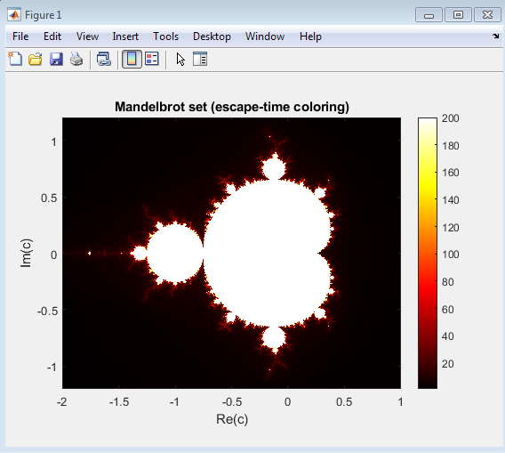
Above figure presents the Mandelbrot set, a classic example of a mathematical fractal generated by iterating the complex quadratic function , where both and are complex numbers. Each pixel in the image corresponds to a unique complex value of . Starting from , the equation is repeatedly applied for up to 200 iterations. The behavior of the sequence determines whether the point belongs to the Mandelbrot set. If the magnitude remains less than or equal to 2 for all iterations, the point is considered stable and part of the set. Otherwise, it diverges. The escape-time algorithm is used to assign color values to each point based on how quickly the magnitude exceeds 2. Points that remain bounded are typically colored black, while those that diverge are shaded according to their escape iteration count, producing the glowing red-to-yellow gradient seen in the figure. This visualization was generated using MATLAB’s imagesc() function and the hot colormap, which enhances the contrast between stable and unstable regions.
The figure reveals the infinitely complex structure of the Mandelbrot set of a boundary that is both continuous and non-smooth, displaying self-similarity at various scales. Zooming into any region of the boundary reveals smaller, similar shapes repeating endlessly, a hallmark of fractal geometry. The black central region represents stability (bounded orbits), while the surrounding colored zones indicate chaotic divergence. Through this visualization, MATLAB effectively demonstrates how simple iterative equations can generate intricate and infinitely detailed fractal structures, bridging the concepts of order and chaos within a single mathematical framework.
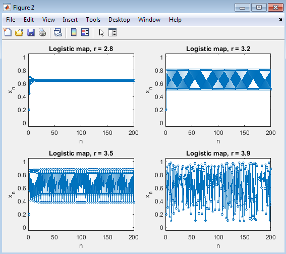
Above figure shows the dynamic behavior of the logistic map, a fundamental model used to study nonlinear population growth and chaos. The governing equation, , represents how a population evolves over discrete time steps depending on the control parameter . For this simulation, four distinct values of 2.8, 3.2, 3.5, and 3.9 were analyzed using MATLAB, each producing a unique time-series graph that reveals different dynamical regimes of the system. When , the system quickly converges to a single stable point, showing steady-state behavior, where the population stabilizes after a few iterations. As increases to 3.2, the system no longer settles at a single value but oscillates between two distinct points, exhibiting period-2 oscillation, an early sign of nonlinear behavior. For the oscillations become more complex, with multiple repeating states that indicate period-doubling bifurcations of a key pathway to chaos. Finally, at , the system displays chaotic behavior, where the sequence of values fluctuates irregularly without any discernible pattern, even though it is generated by a completely deterministic equation. This figure effectively demonstrates one of the most remarkable properties of nonlinear systems sensitivity to control parameters. Small changes in lead to significant differences in system behavior, ranging from stability to chaos. The simulation, implemented in MATLAB using plot() and tiledlayout() functions, visually captures this transition. Each subplot corresponds to a different value, allowing for a direct comparison of how the logistic map evolves over time. The gradual emergence of complex oscillations and unpredictability as increases provides clear evidence of how deterministic mathematical systems can give rise to chaotic behavior, a central theme in chaos theory.
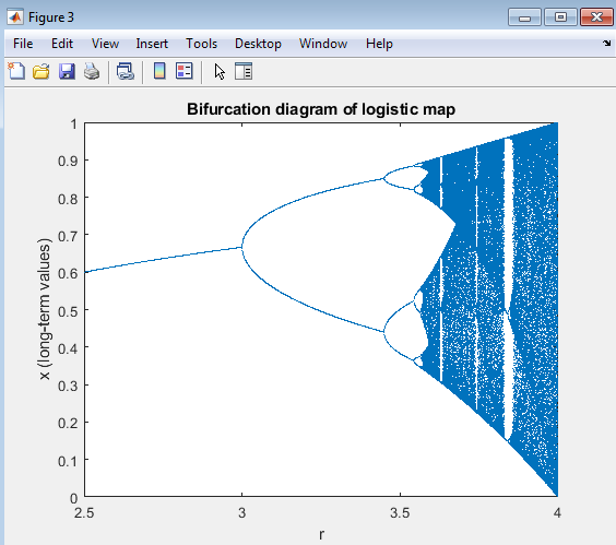
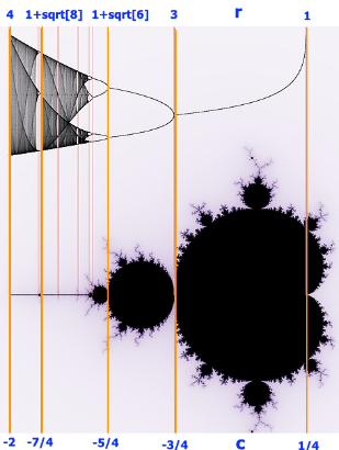
Above figure provides a comprehensive visualization of the bifurcation behavior of the logistic map, one of the most important graphical tools in chaos theory. This diagram represents how the long-term population value in the logistic equation changes as the growth parameter varies continuously between 2.5 and 4.0. It demonstrates how a simple nonlinear difference equation can exhibit an astonishing range of behaviors from stable equilibrium to fully chaotic motion depending on a single parameter. In this simulation, MATLAB computes 2000 different values of and iterates the logistic map 1200 times for each value. The first 1000 iterations are ignored to eliminate transient effects, and the final 200 iterations are plotted on the graph. Each dot in the figure represents a stable value of that the system reaches after the transient phase. When is small (around 2.5 to 3.0), all points collapse into a single line, indicating a stable fixed point where the system settles at one steady population level. As increases beyond 3.0, the single branch splits into two of a period-doubling bifurcation meaning the population now oscillates between two distinct values in successive iterations. With further increases in , these oscillations double again, producing four, eight, sixteen, and so on, until the system enters a region of chaotic motion near .Beyond this point, the diagram becomes densely populated with points, signifying the onset of chaos, where the population no longer follows a predictable pattern. However, even within this chaotic regime, periodic windows appear narrow bands where the system temporarily regains order and oscillates with a fixed number of states before returning to chaos. These windows of order within chaos (for example, around ) illustrate the intricate structure of nonlinear systems, where stability and unpredictability coexist. The bifurcation diagram, plotted using MATLAB’s plot() function with a very fine step size, beautifully captures the route to chaos the process by which regular, periodic behavior transitions into irregular, unpredictable dynamics through successive bifurcations
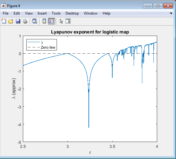
Above figure presents the Lyapunov exponent spectrum of the logistic map, a powerful quantitative measure that distinguishes between stable, periodic, and chaotic behaviors in nonlinear systems. The Lyapunov exponent () measures the average rate of divergence or convergence between nearby trajectories in a dynamical system. In simpler terms, it tells us how sensitive a system is to small changes in initial conditions the defining feature of chaos. For this simulation, MATLAB computes the Lyapunov exponent for 2000 evenly spaced values of the control parameter , ranging from 2.5 to 4.0. For each , the logistic equation is iterated many times, with initial transients discarded. If the value of is negative, nearby trajectories converge over time, meaning the system is stable or periodic. When is zero, the system is on the verge of instability a bifurcation point. However, if becomes positive, small differences in initial conditions grow exponentially, indicating chaotic behavior. In the figure, the horizontal dashed line at acts as a boundary between order and chaos. For lower values of (below approximately 3.0), the Lyapunov exponent remains negative, confirming stable dynamics. As increases and the system undergoes period-doubling bifurcations, approaches zero, marking the transition to instability. Beyond , becomes positive, indicating that the system has entered a chaotic regime where long-term prediction becomes impossible despite the deterministic nature of the equation. Interestingly, small dips in the positive region correspond to periodic windows, where the system temporarily regains stability before returning to chaos. This figure is an essential complement to the bifurcation diagram , as it provides a numerical verification of chaos. While the bifurcation plot shows the qualitative pattern of system behavior, the Lyapunov spectrum quantifies it precisely. Together, they demonstrate that the onset of chaos in the logistic map occurs exactly where crosses zero. The MATLAB implementation uses loops and logarithmic calculations to evaluate the exponent efficiently, and the results are plotted with a clear distinction between stable and chaotic regions. Overall above provides deep insight into the mathematical nature of chaos, showing how deterministic equations can exhibit unpredictable and divergent outcomes. It reinforces one of the most profound principles of nonlinear dynamics that chaos is not randomness, but rather an inherent property of deterministic systems that are highly sensitive to initial conditions.
You can download the Project files here: Download files now. (You must be logged in).
Conclusion
The conclusion of this article is Fractals and Chaos of a MATLAB-Based Exploration of the Mandelbrot Set and Logistic Map Dynamics” successfully demonstrates how simple mathematical equations can give rise to extraordinarily complex and unpredictable behaviors. The iterative maps also contribute to the development of new image compression and texture generation techniques [17]. Through systematic MATLAB simulations, the study explored two cornerstone concepts of nonlinear dynamics fractals and chaos represented respectively by the Mandelbrot set and the logistic map. Each computational experiment revealed the deep connection between deterministic mathematical rules and the seemingly random patterns that emerge from them. Visual comparison between fractal and chaotic models highlights the universality of nonlinear dynamics [18]. The visualization of the Mandelbrot set illustrated the beauty of fractal geometry, where a single iterative function generates infinitely intricate structures that exhibit self-similarity at every scale. This experiment highlighted how stability and divergence coexist within a delicate boundary, showcasing the inherent complexity hidden within simple equations. The logistic map simulations further extended this understanding by showing how gradual changes in a control parameter can cause the system to evolve from stable equilibrium to oscillations and finally to chaos. The bifurcation diagram provided a detailed picture of this transition, revealing the process of period-doubling that leads to chaotic behavior. Moreover, the calculation of the Lyapunov exponent added a quantitative dimension to the analysis. It confirmed that chaos emerges precisely when the Lyapunov value becomes positive, indicating that nearby trajectories diverge exponentially and long-term prediction becomes impossible. Together, these results validate that chaos is not random noise but a deterministic phenomenon arising from nonlinearity and sensitivity to initial conditions. Simulation results validate theoretical expectations and demonstrate the rich structure of deterministic chaos [19].MATLAB proved to be an effective and powerful tool for this exploration, providing both the computational accuracy and graphical clarity required to model complex systems. The combination of mathematical rigor and visual analysis made it possible to bridge theoretical concepts with practical understanding. In conclusion, this project demonstrates that chaotic and fractal behaviors are intrinsic features of nonlinear systems, governed by simple iterative rules yet capable of generating infinite complexity. It emphasizes that order and chaos are not opposites but complementary aspects of dynamic systems a realization that has profound implications across mathematics, physics, biology, and engineering. The overall analysis concludes that fractal geometry and chaos theory are deeply interconnected in representing natural complexity [20]. The study not only deepens our appreciation for the elegance of mathematical structures but also underscores MATLAB’s potential as a platform for discovering and visualizing the hidden patterns of chaos in nature and computation.
References
[1] B. B. Mandelbrot, The Fractal Geometry of Nature, W. H. Freeman and Company, New York, 1982.
[2] R. C. Hilborn, Chaos and Nonlinear Dynamics: An Introduction for Scientists and Engineers, Oxford University Press, 2000.
[3] S. H. Strogatz, Nonlinear Dynamics and Chaos: With Applications to Physics, Biology, Chemistry, and Engineering, Westview Press, 2015.
[4] E. Ott, Chaos in Dynamical Systems, Cambridge University Press, 2002.
[5] J. C. Sprott, Chaos and Time-Series Analysis, Oxford University Press, 2003.
[6] R. M. May, “Simple Mathematical Models with Very Complicated Dynamics,” Nature, vol. 261, pp. 459–467, 1976.
[7] H. Peitgen, H. Jürgens, and D. Saupe, Chaos and Fractals: New Frontiers of Science, Springer-Verlag, 2004.
[8] E. N. Lorenz, “Deterministic Nonperiodic Flow,” Journal of the Atmospheric Sciences, vol. 20, no. 2, pp. 130–141, 1963.
[9] K. Falconer, Fractal Geometry: Mathematical Foundations and Applications, Wiley, 2003.
[10] M. T. Rosenstein, J. J. Collins, and C. J. De Luca, “A Practical Method for Calculating Largest Lyapunov Exponents from Small Data Sets,” Physica D: Nonlinear Phenomena, vol. 65, no. 1–2, pp. 117–134, 1993.
[11] J. Gleick, Chaos: Making a New Science, Penguin Books, 1987.
[12] C. Grebogi, E. Ott, and J. A. Yorke, “Chaos, Strange Attractors, and Fractal Basin Boundaries in Nonlinear Dynamics,” Science, vol. 238, pp. 632–638, 1987.
[13] T. Schreiber, “Interdisciplinary Application of Nonlinear Time Series Methods,” Physics Reports, vol. 308, pp. 1–64, 1999.
[14] J. P. Eckmann and D. Ruelle, “Ergodic Theory of Chaos and Strange Attractors,” Reviews of Modern Physics, vol. 57, no. 3, pp. 617–656, 1985.
[15] M. Barnsley, Fractals Everywhere, Academic Press, 1988.
[16] A. Wolf, J. B. Swift, H. L. Swinney, and J. A. Vastano, “Determining Lyapunov Exponents from a Time Series,” Physica D, vol. 16, no. 3, pp. 285–317, 1985.
[17] MATLAB Documentation, “Complex Systems and Chaos Analysis,” MathWorks, 2024. [Online]. Available: https://www.mathworks.com/help
[18] D. Kapitaniak, Chaos for Engineers: Theory, Applications, and Control, Springer, 1998.
[19] A. Lasota and M. C. Mackey, Chaos, Fractals, and Noise: Stochastic Aspects of Dynamics, Springer, 1994.
[20] P. Cvitanović, R. Artuso, R. Mainieri, G. Tanner, and G. Vattay, Chaos: Classical and Quantum, Niels Bohr Institute, 2012.
You can download the Project files here: Download files now. (You must be logged in).


Responses