

Model-Based Control Design for Swing-Up and Balance of an Inverted Pendulum Using Simulink and Arduino
Abstract
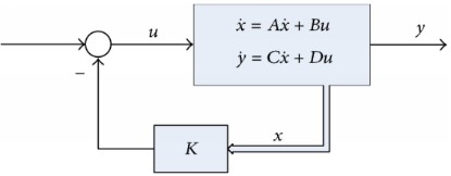
This report presents the design, simulation, and hardware implementation of a model-based control system for swinging up and stabilizing an inverted pendulum using MATLAB/Simulink and Arduino Mega 2560. The control architecture integrates a collocated energy-shaping controller for swing-up and a Linear Quadratic Regulator (LQR) for balancing. The system comprises a pendulum-cart mechanism driven by a DC motor, with position feedback from rotary encoders. The nonlinear dynamic model is derived using Euler-Lagrange equations and validated through simulation. The designed controller is implemented using Simulink’s Arduino support package for real-time operation. Results demonstrate successful swing-up and stabilization from a hanging position, confirming the controller’s robustness and practical feasibility.
Introduction
The inverted pendulum is a classical control problem that represents a highly nonlinear and unstable system, often used for validating modern control strategies in real-time environments [1]. It finds applications in robotics, aerospace, and transportation systems where balance and stability are critical [2]. The dual-objective control problem involves first swinging the pendulum from its stable downward position to an upright one (swing-up control) and then maintaining it at the unstable equilibrium (balancing control) [3]. Traditional PID controllers fail to manage this task due to the system’s nonlinearities and underactuation, necessitating more advanced model-based strategies [4].
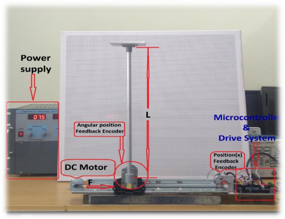
The task is to balance a simple pendulum around its unstable equilibrium, using only horizontal forces on the cart. The Inverted Pendulum setup, shown in Fig.1, consists of a Linearguide that is taken out from defective Inkjet Printer. This linear guide further modified by adding two Encoders for the measurement of both Linear & angular position. The Microcontroller we use is Arduino Mega2560.Cytron 10Amp DC motor Driver is used to drive a motor.
1.1 Inverted Pendulum Components
The component of the Inverted Pendulum module are listed in Table 1 and labelled in Fig.1.
Table 1: Inverted Pendulum components
| Sr.No. | Component |
| 1. | Linear Guide taken out from Inkjet Printer. |
| 2. | Pendulum Aluminium Rod. |
| 3. | Encoders 600PPR. |
| 4. | USB A/B Printer Cable 3.0/2.0 (High speed). |
| 5. | Arduino Mega2560. |
| 6. | Cytron 10Amp DC motor drive (MD10C R3). |
1.2 Nomenclature
Table 2: Inverted Pendulum system specifications.
| Symbol | Description | Matlab Variable | Value with Units |
| M | Mass of the pendulum rod. | M | 0.1 kg |
| MC | Mass of the Cart | M_c | 0.135 Kg |
| L | Pendulum length from pivot to centre of gravity | L | 0.2 m |
| Jm | Motor rotor moment of inertia | Jm | 3.26×10-08 kg.m2 |
| Rm | Motor armature resistance | Rm | 12.5 Ω |
| kb | Motor back emf constant | Kb | 0.031 V/rad/sec |
| kt | Motor torque constant | Kt | 0.031 N.m/A |
| R | Motor pinion radius | R | 0.006 m |
| B | Viscous damping at pivot of pendulum | B | 0.000078 N.m/rad/sec |
| C | Viscous friction coefficient for cart displacement | C | 0.63 N/m/sec |
| I | Mass moment of inertia of pendulum rod | I | 0.00072 kg.m2 |
| M | Total cart weight mass including motor inertia | M | 0.136 kg |
| G | Gravitational constant | G | 9.81 m/sec2 |
Nomenclature
Where:
𝐽𝑚
𝑀 = 𝑀𝑐 + 𝑟2
- 𝑇 = Total Kinetic energy of the
- 𝑈 = Total potential energy of the
- 𝑥𝑝 = absolute 𝑥 – coordinate of the pendulum centre of
- 𝑦𝑝 = absolute 𝑦 – coordinate of the pendulum centre of
The following topics will be covered in this experiment:
- Modeling the dynamics of the Inverted Pendulum using Euler-Lagrange
- Obtaining a Linear state-space representation of the
- Design a Energy based nonlinear swing upstrategy for the Inverted
- Designing a state-feedback control system that balances the pendulum at its vertical upward position using
- Implementing the Digital LQR controller on Arduino Mega2560 Controller via Matlab Simulink.
Design Methodology
2.1. Hardware Setup
The pendulum-cart system is constructed using a linear guide rail from a discarded inkjet printer, a DC motor, a Cytron MD10C R3 motor driver, and an Arduino Mega 2560 microcontroller. Angular and linear positions are measured using rotary encoders interfaced with Arduino. The motor driver provides high current handling and directional control via PWM and logic signals from the Arduino. MATLAB/Simulink is used for control logic design and code generation [5].
2.2. Modeling
The dynamics of the inverted pendulum system are derived using Euler-Lagrange equations. The state variables include the cart position, pendulum angle, and their respective velocities. The derived nonlinear equations are verified using symbolic computation and simulated in MATLAB. For balance control design, the model is linearized about the upright position using Jacobian linearization to obtain a state-space model [6].
2.3. Swing-Up Controller
The swing-up phase utilizes a Partial Feedback Linearization (PFL) strategy. This energy-based method regulates the system’s total mechanical energy by injecting energy into the pendulum until it reaches a homoclinic orbit (i.e., zero velocity at the vertical position) [7]. The swing-up controller applies torque by manipulating the cart’s acceleration, ensuring the pendulum gains sufficient kinetic energy for transition.
2.4. Balance Controller (LQR)
Once the pendulum nears the upright position, a Linear Quadratic Regulator (LQR) takes over. The LQR minimizes a cost function defined by weighted state deviations and control effort, providing optimal feedback gains for stabilization. The switching condition is based on the pendulum angle threshold (e.g., within ±15 degrees of vertical) [8].
2.5. Mathematical Modeling of IP system(EOM)
The Equation of Motion is obtained by fig.2:
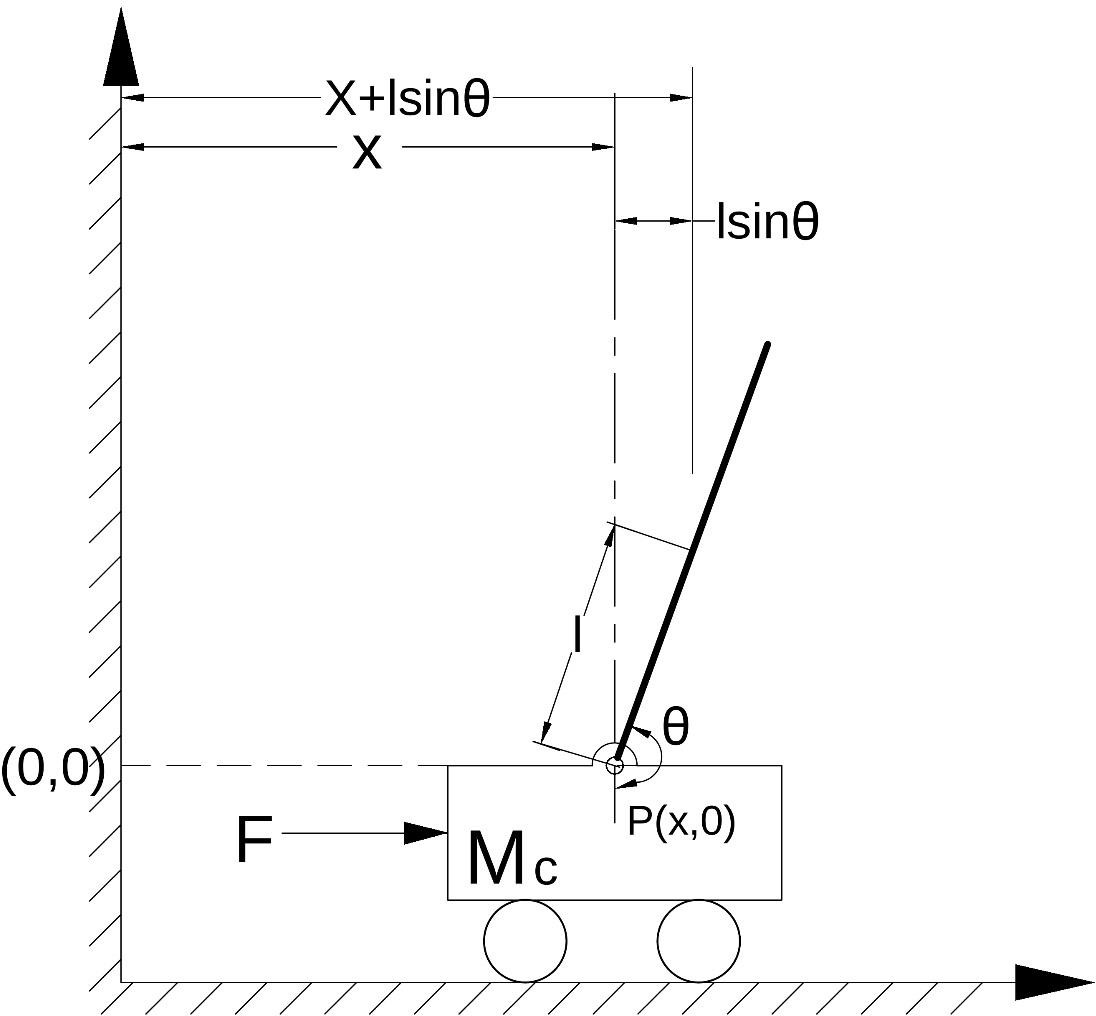
Kinematics of the system
The non-relativistic Lagrangian for a system of particles can be defined by
ℒ = 𝑇 − 𝑈 | (2) |
Total Potential energy of the system:
𝑈 = −𝑚𝑔𝑙 cos 𝜃 | (3) |
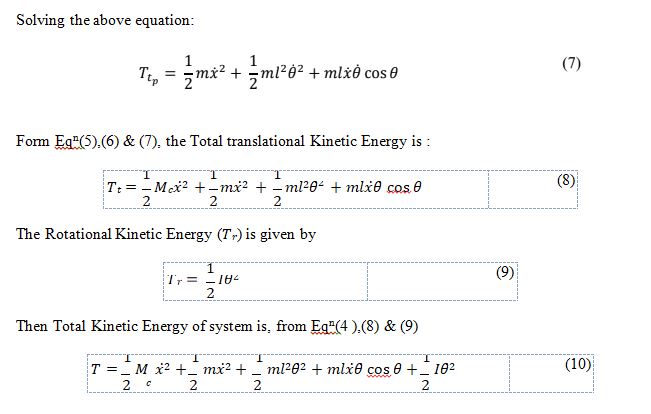
Total Kinetic Energy of the system is the sum of ‘Translational (𝑇𝑡)’ & ‘Rotational (𝑇𝑟)’ Kinetic Energy:
𝑇 = 𝑇𝑡 + 𝑇𝑟 | (4) |
You can download the Project files here: Download files now. (You must be logged in).
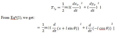
The Total Translational kinetic energy (𝑇𝑡) is given by
𝑇𝑡 = 𝑇𝑡𝑐 + 𝑇𝑡𝑝 | (5) |
The translational kinetic energy (𝑇𝑡𝑐) of cart is given by:
The translational kinetic energy (𝑇𝑡𝑝) of the pendulum is the given by:
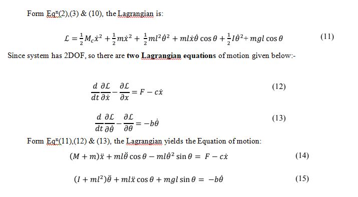
2.5. Simulink Implementation
Simulink models are constructed for both the nonlinear plant and the controller logic. Using the Arduino Support Package, the code is deployed in real-time to the Mega 2560. The swing-up and balance controllers are implemented as subsystems with a condition-based switching logic. Real-time feedback from encoders is fed into the Simulink model via serial communication blocks [9].
Simulation of Nonlinear dynamics of Inverted Pendulum:
Simulation of above Eqsn(14) & (15), we get
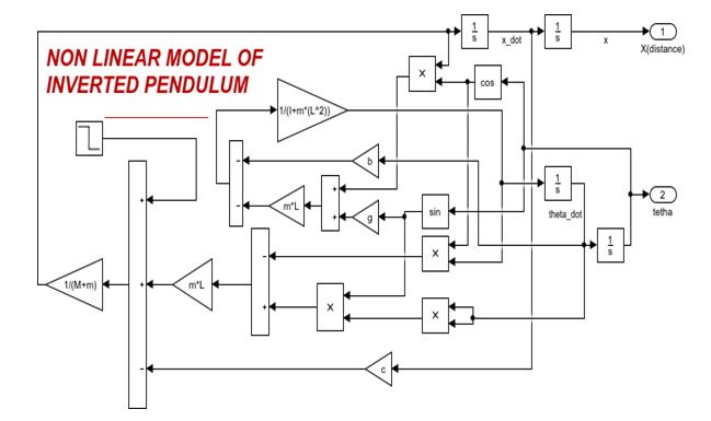
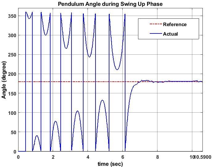
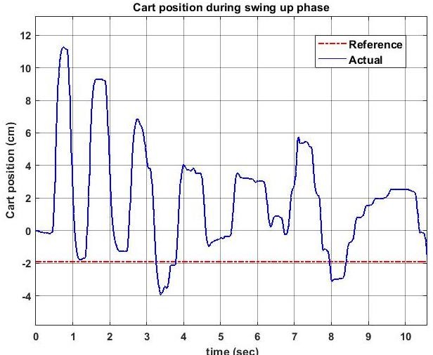
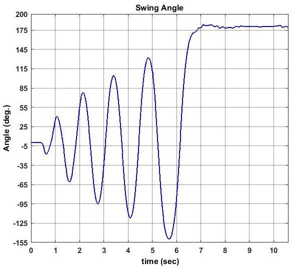
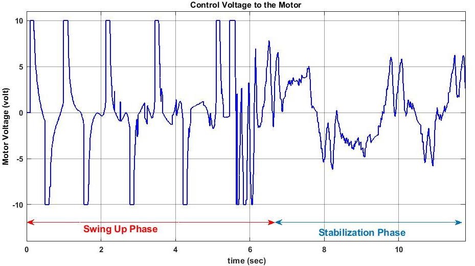
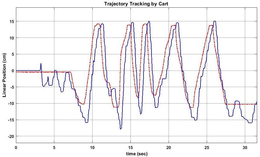
3.1 Results
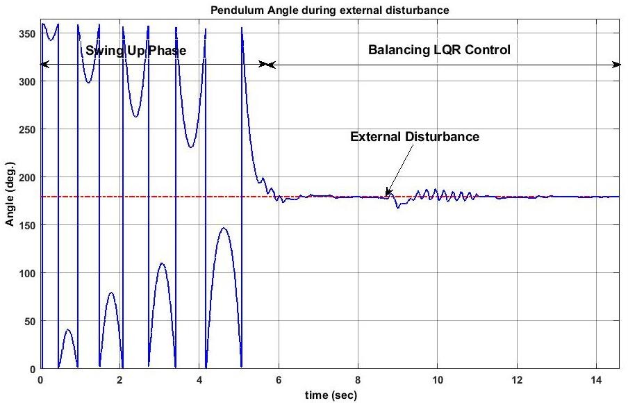
The integrated system was tested for multiple initial conditions with the pendulum hanging freely. The swing-up controller successfully elevated the pendulum to the upright position within 3-5 seconds, depending on initial energy. The LQR controller was able to stabilize the pendulum with minimal overshoot and sustained oscillations, confirming robust feedback performance. Simulation results closely matched the hardware response, with only minor discrepancies due to motor friction and encoder noise. Power consumption and control effort were within acceptable limits. Data logging confirmed real-time capability of Simulink-Arduino integration for educational and research applications [10].
You can download the Project files here: Download files now. (You must be logged in).
4. Inverted Pendulum Swing Up controller design
In this section a control scheme is developed for swinging up the pendulum from its vertical downward position. The controller is an energy based controller.
Energy based controller simply control the total amount of the energy in the system such as adding enough energy, the pendulum is swing up from the hanging position to its unstable equilibrium point.
Many different control algorithms can be used to perform the swing up control such as, trajectory tracking, rectangular reference input swing up type. The energy shaping controller tend to be the most natural to derive and perhaps the most well–known.
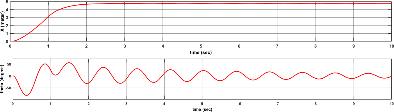
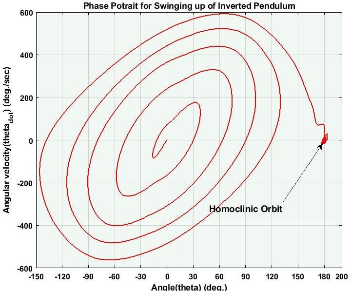
(a). Homoclinic Orbit
For a simple pendulum phase portrait, the orbits of this phase plot are defined by countours of constant energy. One very special orbit, known as Homoclinic Orbit, is the orbit which passes through the unstable fixed point. In below figure Red orbit is Homoclinic orbit.
Fig.5 Phase portrait of simple pendulum motion with undamped & unactuated system
(b). Nonlinear Control Law Formulation by using Collocated Partial Feedback Linearization
We seek to design a nonlinear feedback control policy which drives the simple pendulum from any initial condition to the unstable fixed point, a very reasonable strategy would be to use actuation to regulate the energy of the pendulum to place it on this homoclinc orbit. The basic idea:
- Use collocated Partial Feedback Linearization to simplify the
- Use Energy shaping to regulate the pendulum to it’shomoclinc
- Then to add a few term to make sure the cart stays near the
Differentiating with respect to time we obtain:
𝐸̃̇ = 𝐸̇ = (𝐼 + 𝑚𝑙2)̇𝜃̈ + 𝑚𝑔𝑙 sin 𝜃𝜃̇
Put the value of 𝜃̈ from Eqn(24), into above Eqn: We get,
𝐸̃̇ = −𝑏𝜃̇2 − 𝑚𝑙𝑢𝜃̇ cos 𝜃
Therefore, if we design a controller of the form
𝑢 = 𝑘𝜃̇ cos 𝜃 𝐸̃, 𝑘 > 0
Then the resulting error dynamics are:
𝐸̃̇ = −𝑏𝜃̇2 − 𝑚𝑙𝑘𝜃̇2 cos2 𝜃 𝐸̃, The damping term 𝑏 is very small, then we can neglect this, These error dynamics imply an exponential convergence:
𝐸̃ → 0,
Except for states where 𝜃̇=0. The essential property is that when 𝐸 >𝐸𝑟, we should remove energy from the system (damping) and when 𝐸 <𝐸𝑟, we should add energy (negative damping).
Even if the control action are bounded, the convergence is easily preserved.
However for energy to change quickly the magnitude of the control signal must be fairly large. As a result a tunable gain k is multiplied by the above and the controller is saturated at the maximum acceleration deliverable by the motor 𝑢𝑚𝑎𝑥 ∶
𝑢 = 𝑠𝑎𝑡𝑢𝑚𝑎(𝑘(𝐸 − 𝐸𝑟)𝑆𝑖𝑔𝑛(𝜃̇ cos 𝜃)) (27) From Eqn(27) &Eqn(23),
Collocated Partial Feedback Linearizationcontrol law, that is the appropriate Nonlinear Control Law in term of Force.
& from Eqn(21),We get the relation between Control Voltage & applied Force.
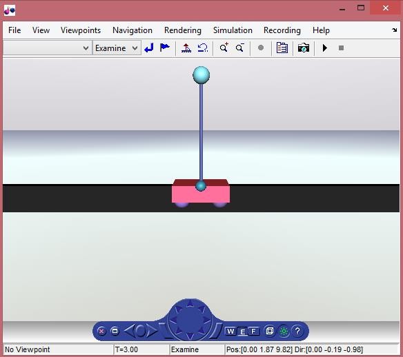
3D VRML Model of Inverted Pendulum:
5. LQR balanced Control Design
Stability Test:
To check the stability means to analyze whether the open-loop system (without any feedback) is stable or not. The eigenvalues of the system state matrix, ‘A’, can determine the stability. That is equivalent to finding the poles of the transfer function of the system.
𝐴𝐼 = ⋋ 𝐼.
Where ⋋ is the eigenvalue and 𝐼 is the eigenvector.The eigenvalues tell us how the matrix A “acts” in different directions (eigenvectors).
The eigenvalues of the 𝐴 matrix are the values of s where det(𝑠𝐼 − 𝐴) = 0.A system is stable if real part of all its eigenvalues must be lied in the left- half of the s-plane such as negative number.
>> Poles = 𝑒𝑖(𝐴)
ans =
0
-19.6327
6.9178
-5.6006
You can download the Project files here: Download files now. (You must be logged in).
Controllability Test:
Complete state controllability (or simply controllability if no other context is given) describes the ability of an external input to move the internal state of a system from any initial state to any other final state in a finite time interval.
Controllability Matrix
For LTI (linear time-invariant) systems, a system is reachable if and only if its controllability matrix, ζ, has a full row rank of p, where p is the dimension of the matrix A, and p × q is the dimension of matrix B.
ζ = [𝐵 𝐴𝐵 𝐴2𝐵 … … 𝐴𝑝−1𝐵] ∈ 𝑅𝑝 𝑥 𝑝𝑞
A system is controllable when the rank of the system matrix A is p, and the rank of the controllability matrix is equal to:
𝑅𝑎𝑛(ζ) = 𝑅𝑎𝑛𝑘(𝐴−1ζ) = 𝑝
MATLAB allows one to easily create the controllability matrix with the ctrb command. To create the controllability matrix ζ simply type:
≫ ζ = ctrb(A, B);
≫ Rank = rank(ζ);
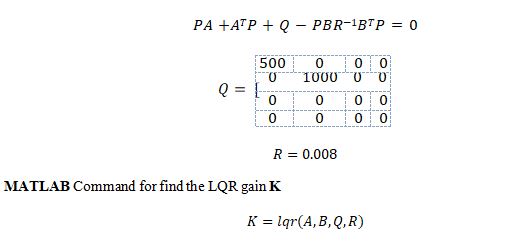
Optimal Full State Feedback Control Law:𝑚 = −𝐾𝑋
𝐾 = 𝑅−1𝐵𝑇𝑃
𝑉𝑚 = −𝑅−1𝐵𝑇𝑃𝑋
𝑃is the solution of Algebraic Riccati Equation:
6. Result Discussion:
The Experimental results are showing in graphs to illustrate that the Swing Up& LQRcontroller are working well with desire control specifications.
Results are listed below:
7. In-Lab Procedures
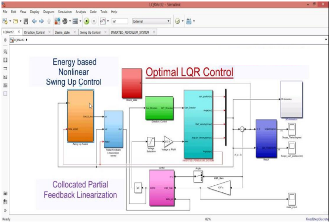
The LQRArd Simulink diagram shown in Fig.5 is used to control the IP system using the Arduino support package. The INVERTED_PENDULUM_SYSTEM subsystem contains Arduino block that interface with the DC motor and sensors (encoders) of the IP system.
Follow these steps to implement a complete control system on the actual IP plant:
- Load the MATLAB
- Browse through the current Directory window in MATLAB and find the folder than contains the controller files.
- Double-click on the slx file to open the Simulink diagram shown in Fig.5.
- Double-click on the m to open the setup script for this same.
- Double-click on the m to load Rensselaer Arduino Support package in Simulink library.
8. Conclusion
This project successfully demonstrates the application of model-based control techniques for swinging up and stabilizing an inverted pendulum system. The use of energy-based PFL for swing-up and LQR for balance proved effective both in simulation and physical hardware implementation. The project highlights the usefulness of MATLAB/Simulink for rapid prototyping and controller testing in embedded systems. Future work may include implementing adaptive controllers to compensate for parameter variations and disturbances.
References
- Astrom, K. J., & Furuta, K. (2000). Swinging up a pendulum by energy control. Automatica, 36(2), 287-295.
- Spong, M. W. (1995). The swing up control problem for the acrobot. IEEE Control Systems Magazine, 15(1), 49-55.
- Ogata, K. (2010). Modern Control Engineering. Prentice Hall.
- Khalil, H. K. (2002). Nonlinear Systems. Prentice Hall.
- MATLAB and Simulink Hardware Support. (2024). MathWorks. https://www.mathworks.com/hardware-support.html
- Siciliano, B., Sciavicco, L., Villani, L., & Oriolo, G. (2010). Robotics: Modelling, Planning and Control. Springer.
- Fantoni, I., & Lozano, R. (2002). Non-linear Control for Underactuated Mechanical Systems. Springer.
- Bryson, A. E., & Ho, Y. C. (1975). Applied Optimal Control: Optimization, Estimation, and Control. Taylor & Francis.
- Rensselaer Arduino Support Package. (2023).
- Mahony, R., & Hamel, T. (2005). A geometric nonlinear observer for simultaneous localization and mapping. IEEE Transactions on Robotics, 21(4), 730-741.
You can download the Project files here: Download files now. (You must be logged in).


Responses