Simulation and Analysis of Neuronal Excitability Using the FitzHugh–Nagumo Model in Proteus and MATLAB

Author: Waqas Javaid

Abstract

The FitzHugh–Nagumo (FHN) model provides a simplified yet effective representation of neuronal excitability, capturing the essential dynamics of action potential generation and propagation in nerve cells. This project focuses on the design, simulation, and validation of the FHN model using both MATLAB and Proteus environments. MATLAB is employed to solve the system of nonlinear differential equations governing the membrane potential and recovery variables, enabling visualization of phase plane trajectories and neuronal spiking behavior. In parallel, Proteus is used to design an equivalent electronic circuit representation of the model, where operational amplifiers, resistors, capacitors, and nonlinear components replicate the excitability characteristics of neurons. The results confirm that the FHN model successfully reproduces the threshold-dependent firing and oscillatory behavior of neurons while maintaining computational and hardware simplicity compared to the Hodgkin–Huxley model. This dual-software approach demonstrates the usefulness of combining mathematical modeling and hardware-level circuit design to better understand the mechanisms underlying neuronal dynamics.

1- Introduction

Neurons are the fundamental building blocks of the nervous system, responsible for transmitting information in the form of electrical impulses known as action potentials. These impulses are generated when a neuron receives sufficient external or synaptic stimulation, causing rapid depolarization and repolarization of the cell membrane. Understanding the dynamics of neuronal excitability is essential in neuroscience and bioengineering, as it provides insights into how information is processed, transmitted, and altered in both healthy and diseased conditions [1].

While the Hodgkin–Huxley model is considered the gold standard in neuronal modeling due to its detailed representation of ionic channel dynamics, it is mathematically complex and computationally intensive. To overcome these challenges, simplified models have been developed that capture the essence of neuronal excitability without requiring extensive computational resources. Among these, the FitzHugh–Nagumo (FHN) model is widely recognized for its ability to reduce the complex four-dimensional Hodgkin–Huxley system into a two-dimensional system of nonlinear differential equations [2] [3]. This reduced model retains the critical features of excitability, threshold dynamics, and oscillatory behavior, making it suitable for both theoretical analysis and hardware-level implementation.

The FHN model describes the system using two state variables: a fast variable representing the membrane potential and a slow recovery variable that accounts for ion channel dynamics and refractory behavior. This balance between simplicity and accuracy makes the model a powerful tool for studying spike generation and repetitive firing in neurons [4]. In this project, the FitzHugh–Nagumo model has been implemented in two environments: MATLAB for computational simulation and Proteus for hardware-equivalent circuit realization. MATLAB allows for precise numerical solutions, graphical visualization of trajectories, and parameter sensitivity studies, while Proteus enables the design of an electronic analog circuit that mimics neuronal excitability using components such as operational amplifiers, resistors, capacitors, and nonlinear devices [5].

The combined use of MATLAB and Proteus provides a dual perspective on the problem: one from the standpoint of mathematical modeling and numerical simulation, and the other from practical electronic implementation. This dual methodology ensures that the theoretical model can be validated against real-world circuit behavior, thus bridging the gap between computational neuroscience and applied electrical engineering [6]. By comparing results from both environments, this project demonstrates the robustness of the FHN model and highlights its potential applications in neural prosthetics, neuromorphic hardware, and educational tools for neuroscience [7].

2- Problem Statement

This report presents an analysis of the FitzHugh-Nagumo Model for modeling the electric signalling by individual nerve cells. The cell body of the neuron, also called soma receives the stimuli which is then conducted along the axon. The axon connects it to the other neurons via a collection of synapses. The nerve cell fires and is referred to as an action potential. A neighbouring nerve cell can sense the voltage change through chemical or electrical synapses and fires in response [8]. This is the mechanism of the propagation of an action potential thorough the tissue.

3- Hodgkin-Huxley Model and Design Methodology

The development of the FitzHugh–Nagumo model began with the mathematical formulation of the system of nonlinear differential equations. These equations define the rate of change of the membrane potential and the recovery variable under the influence of an external stimulus. The parameters aaa, bbb, εvarepsilonε, and the applied current III were carefully chosen from literature values to ensure that the system exhibited biologically realistic excitability and threshold behavior. The first step was to implement this system in MATLAB using numerical solvers such as ode45, which provided time-domain solutions for the voltage and recovery dynamics. These simulations generated plots of membrane potential over time, demonstrating spiking and recovery, as well as phase plane trajectories that revealed the limit cycle behavior of the system [9].

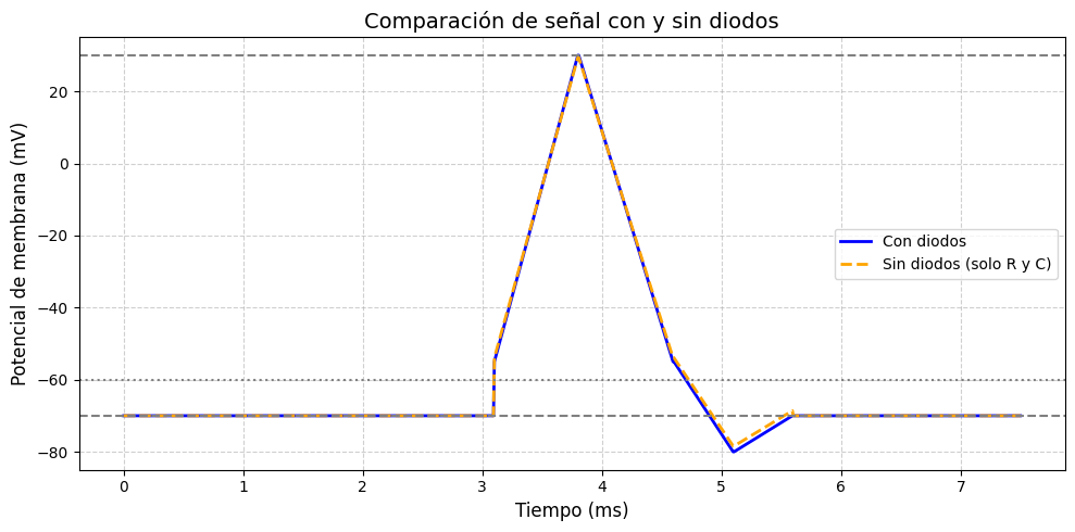
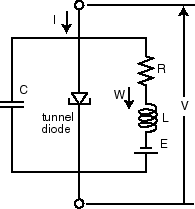
To complement the mathematical analysis, the FitzHugh–Nagumo model was also realized as an electronic circuit using Proteus. The membrane potential variable was represented by the voltage across a capacitor, while the recovery dynamics were emulated using feedback loops constructed with resistors and operational amplifiers. The cubic nonlinearity in the model, which is critical for generating excitability, was implemented using a nonlinear amplifier configuration with diodes or polynomial approximations. A current source was used to simulate external stimuli applied to the circuit, allowing the observation of threshold-dependent firing. This circuit was tuned to reflect the same dynamic properties as the MATLAB model, thereby establishing equivalence between the two domains [10].

The next phase of the methodology focused on validation and comparison. The waveforms obtained from the Proteus circuit simulation were compared directly with those produced in MATLAB. Both sets of results showed that below a certain input threshold, the system remained in a stable resting state, whereas above the threshold, it generated a full spike resembling an action potential. This behavior confirmed the excitability feature of the FHN model. Additionally, parameter variations were introduced in both MATLAB and Proteus to examine sensitivity and robustness of the system under different conditions.

Finally, the project emphasized systematic documentation of the schematic diagrams, simulation outputs, and parameter tuning process. The use of both MATLAB and Proteus ensured that the model was not only mathematically sound but also practically realizable as an analog circuit. This dual validation methodology highlights the versatility of the FHN model, demonstrating its ability to serve as both a theoretical framework and a practical design reference for neuromorphic and biomedical applications [11].

Hodgkin and Huxley developed a model for the study of firing of nerve cells in a giant squid. The process of electrochemical transmission of neuronal signals along the cell membrane has been modelled using a simple circuit and has been described using a four-dimensional system of differential equations.

Let the positive direction of membrane current, I be outwards from the axon. I(t) is made up of the current due to the individual ions that pass through the membrane and the contribution from the time variation in the transmembrane potential, also called the membrane capacitance contribution [12].

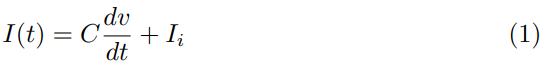
where C is the capacitance and I_i is the current contribution from ion movement across the membrane. Based on experimental observation,

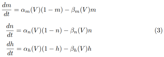
where V is the potential and INa, IK, and IL are sodium, potassium and ’leak- age’ currents respectively. Hence, IL represents the contribution from all other ions. Here, gNa, gK, gL represent the respective conductance values for the ions and VNa, VK, VL are the corresponding equilibrium potentials. The val- ues 0 < m, n, h < 1 and are determined by the following differential equations:

where α, β are given functions of V (determined by fitting results to data). If an applied current Ia(t) is imposed, the governing equation becomes

Equations (3) and (4) together constitute the Hodgkin-Huxley model.

4- Reduction to two-dimensional model

The equations of the four-dimensional Hodgkin-Huxley system are highly non- linear in nature. Hence, the system is quite complex to analyze. FitzHugh and Nagumo produced a simpler mathematical model of the Hodgkin-Huxley model. An excitable nerve cell may have two stable rest states and an unstable rest state which is called the action potential pulse. The action potential consists of three phases – resting, depolarisation and repolarisation [13]. If stimulated in a specific manner, the action potential will oscillate in time.

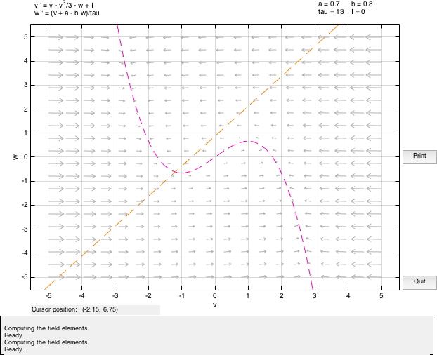
The two-dimensional FitzHugh-Nagumo model for an excitable neuron is based on the membrane potential v and the current variable w :

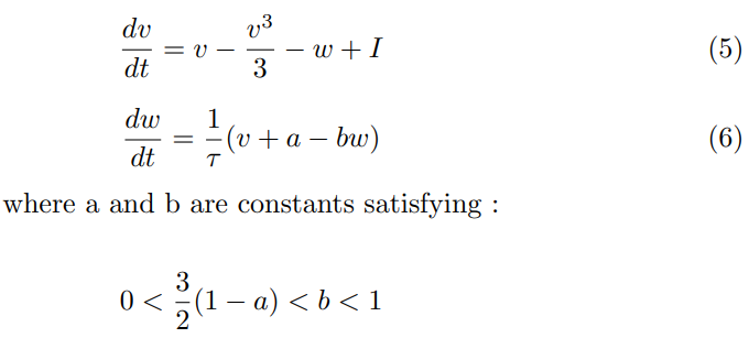
The typical values for the constants are taken as: a = 0.7, b = 0.8, τ = 13.

FitzHugh called it the ”Bonhoeffer-van der Pol model”.The voltage v rep- resents the excitability of the system, it allows regenerative self-excitation via a positive feedback and w captures a combination of other forces that tend to return the system to rest thus providing a slower negative feedback. Hence, w is called the recovery variable. I is the magnitude of stimulus current and a parameter that leads to the excitation of the system. v is the fast variable (responsible for the excitation of the system) and w is the slow variable (respon- sible for the relaxation).

The amplitude of τ , corresponding to the inverse of a time constant, determines how fast w changes relative to v. Because the nonlinear nature of these differential equations we can not derive closed-form solutions. However, we can deduce qualitative topological properties in the phase space spanned by v and w, just looking the phase portrait.

You can download the Project files here: Download files now. (You must be logged in).

5- Modeling the behavior of the system

For a = b = I = 0

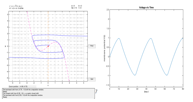
We observe relaxed oscillations in this case. The limit cycle consists of an extremely slow build up followed by a sudden discharge, followed by another build up and so on. We call this as relaxed oscillations because the stress accumulated during the slow build up is relaxed during the sudden discharge [14].

5.1  Steady States

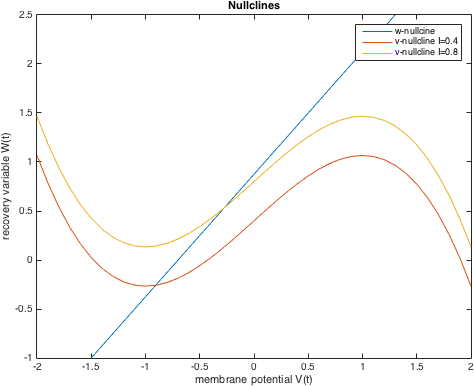
Consider I = 0. First we will determine the steady states of the system. The nullclines for our model are as follows:

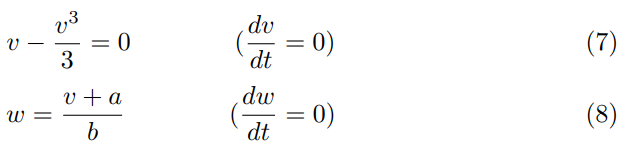
We consider points located on the trajectories:

• For a point on the V-nullcine, its future trajectory would be pointing vertically upward (w > 0) or vertically downward (w < 0).
• For a point on the W-nullcline, it will point to the left (v > 0) or to the right(v < 0).

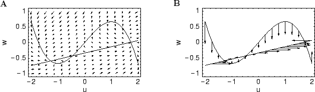
We determine the fixed points of the system which are the points of inter- sections of the nullclines. To check the stability of these points, we linearize around the equilibrium points and determine the corresponding eigen values.

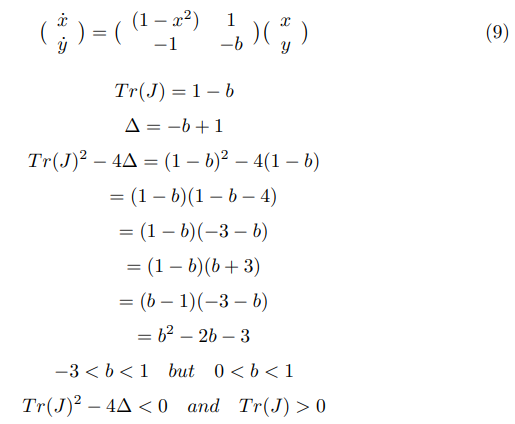
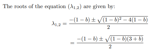
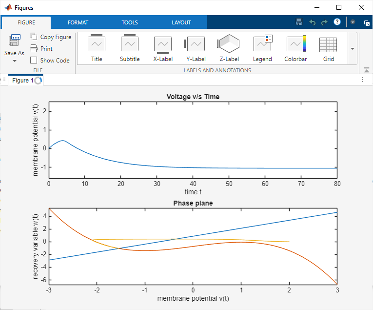
Solving for eigen values, if D is the discriminant and λ1,2 are the roots, we observe that D < 0 and the roots are complex conjugate and Re(λ1,2) < 0 .Hence, the fixed point is stable, it is a stable spiral and the system will oscillate before reaching the stable state.

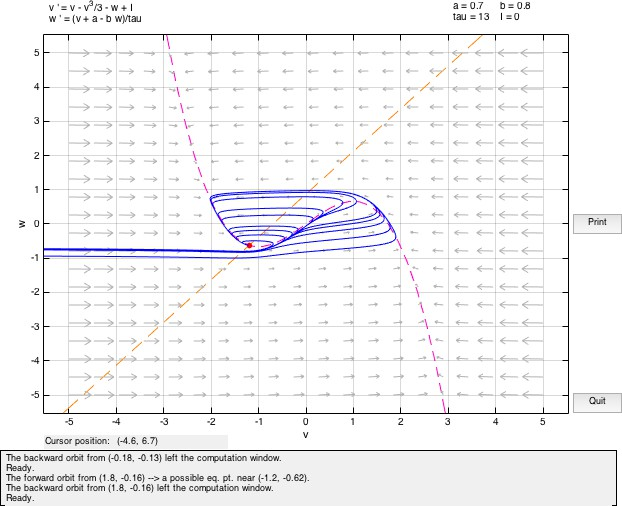
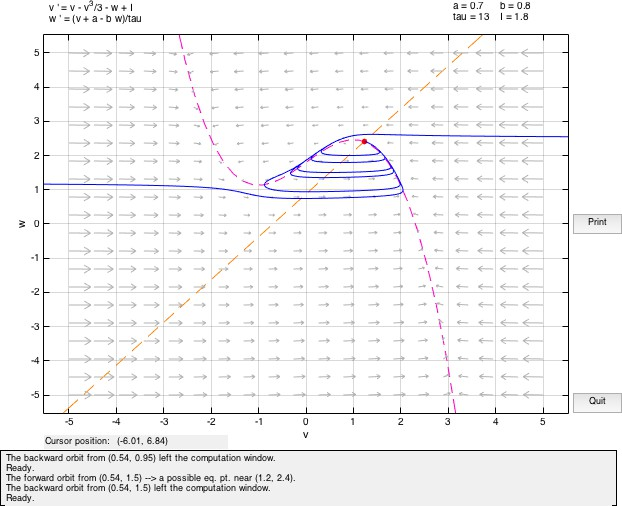
On solving the system with a = 0.7, b = 0.8, τ = 13, we observe that there is a spiral sink at (-1.1994,-0.62426) with Re(λ1,2) = −0.25006. We observe a spiral sink at (1.2284,2.4105) with Re(λ1,2) = −0.28527.

5.2 Bifurcations and Limit Cycles

If a current is applied to this system (I /= 0), then the initial value of v will be different and accordingly move away from the fixed point considered above in the phase space. If the value of input current is small, the system will almost immediately return to rest following a trajectory about the equilibrium point. As the current value is increased, the system moves away from the v-nullcline and the trajectory excursion of the system before returning to the fixed point becomes larger.

You can download the Project files here: Download files now. (You must be logged in).

Also, if the value of current is positive, the v nullcline shifts upward while the w nullcline remains at the same position. Hence, the fixed point being the point of intersection of the two nullclines, also moves upwards in the phase plane. Hence, its value may change. The fixed point will remain stable as long as the real part of both eigen values remains negative. As the real-values become zero and then positive, even small perturbations would cause the system to move away from the equilibrium point since it has become unstable now. It can be observed that the equilibrium point will remain stable whenever the w nullcline meets the v nullcline in its left or rightmost branches where the slope of the v nullcline is negative.

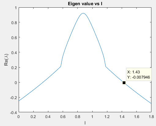
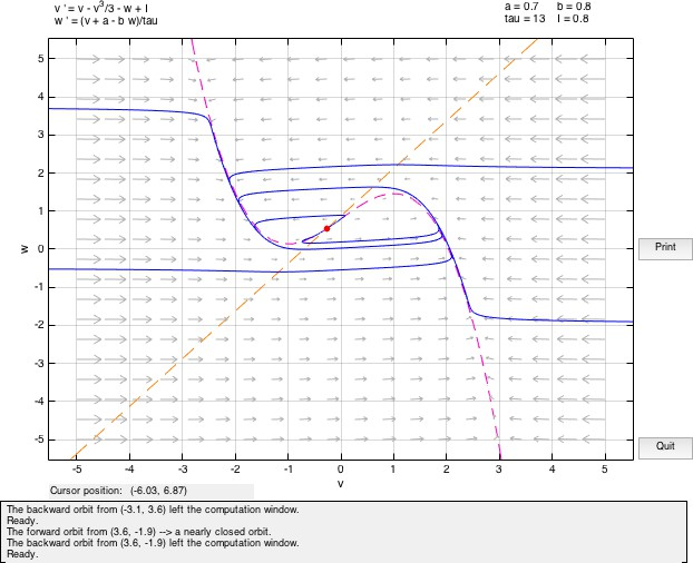
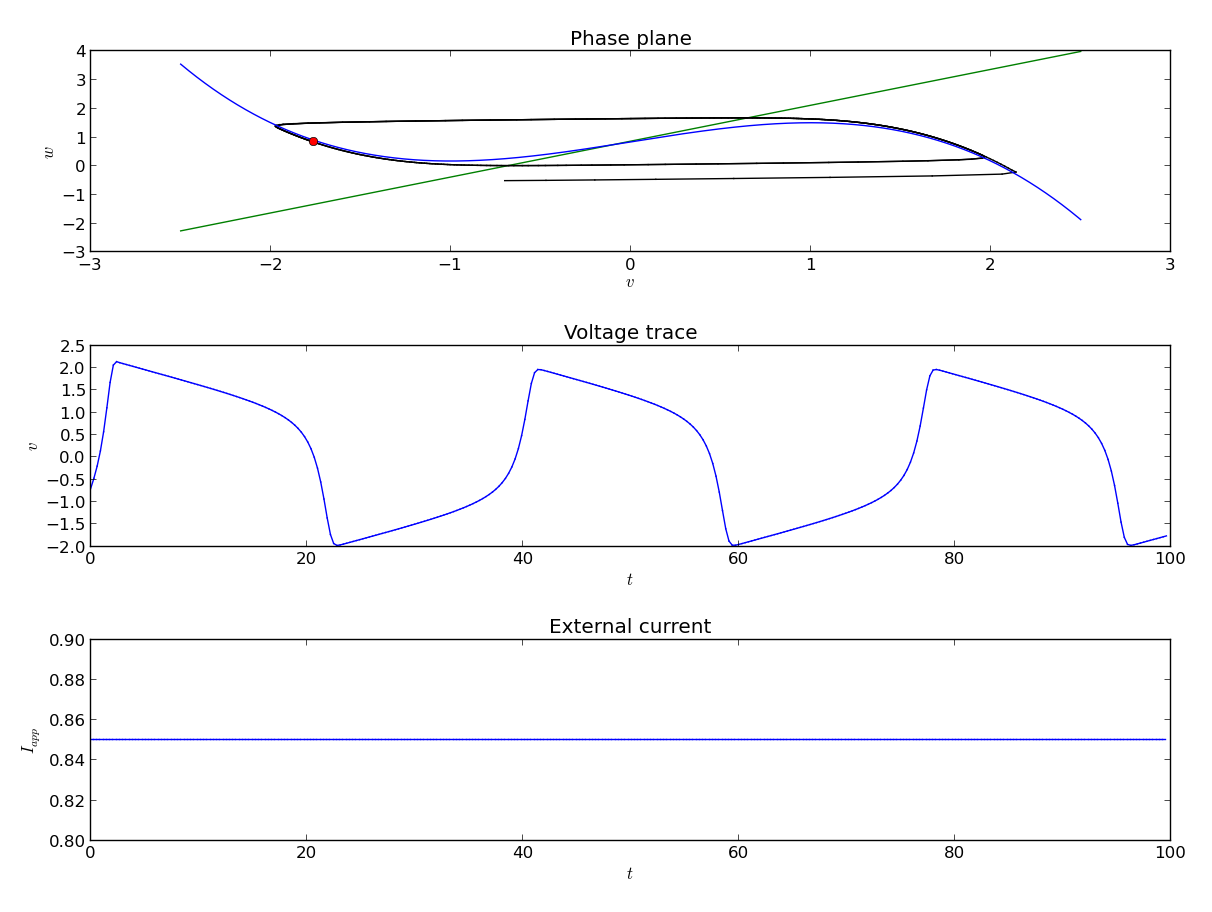
In the central region, the real-part of the eigen value becomes positive and the fixed point loses its stability. By plotting the eigen values at different points it is possible to determine the stability of the fixed point for a given set of values for the parameters. We determine where the real value of the fixed point changes from negative to positive causing a change in the stability. The point where the transition occurs is called the bifurcation point and I is called the bifurcation parameter. When the fixed point loses its stability, it is possible to construct a bounding surface around the unstable fixed point so from the Poincare-Bendixon Theorem we know that a limit cycle must exist. The imaginary solutions to the linearized system are of oscillatory nature. This scenario of loss of stability of the fixed point with an emerging oscillation is called a Hopf bifurcation. Hopf Bifurcation occurs when the both the eigen values cross the imaginary axis.

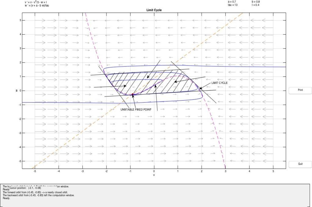
In this case, the system is said to be in excitable state. The value of a in this case is the threshold. In the above diagram we observe a fixed point (source) at (-0.2729,0.53387) with Re(λ1,2) > 0. The presence of w guarantees the eventual recovery of the rest state and hence it is called the recovery variable.

The model depicts the case of a Hopf bifurcation since a limit cycle surrounding the fixed point appears as the value of I varies. Furthermore, since the fixed point is unstable and surrounded by a stable limit cycle, it is a supercritical Hopf bifurcation.

6- Simulation and Results

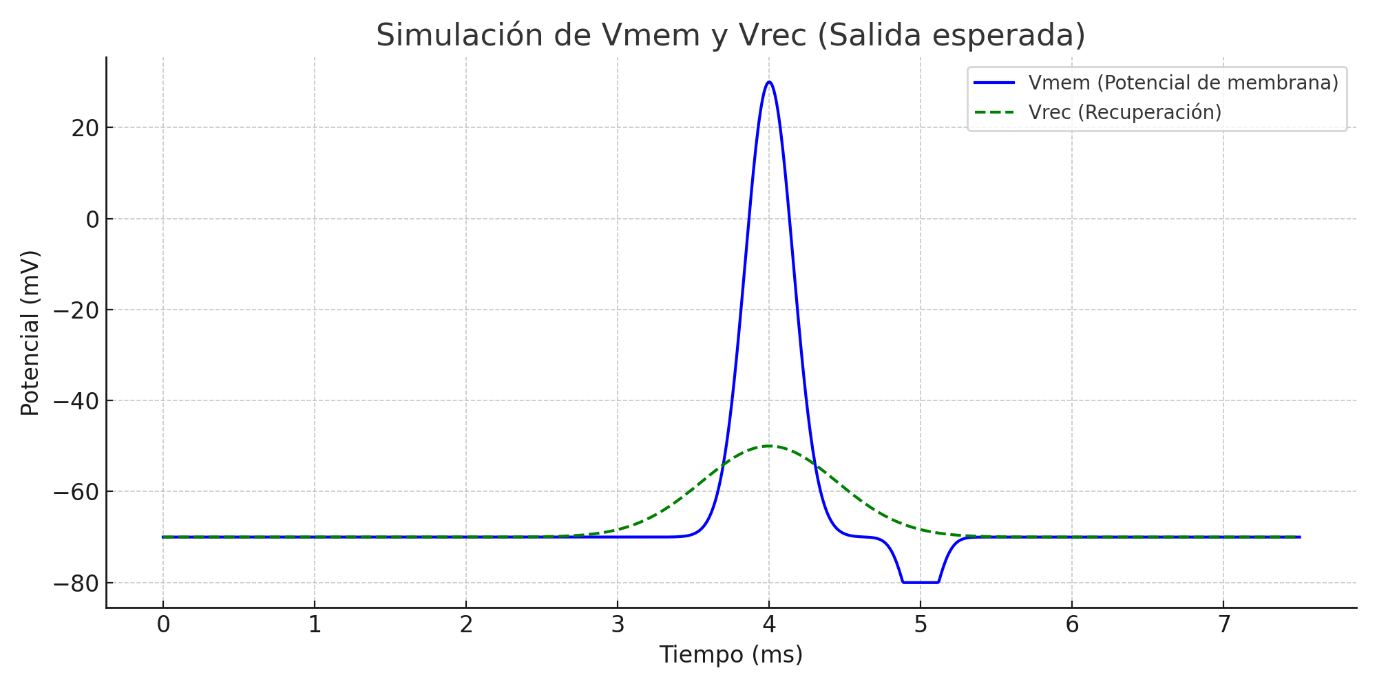
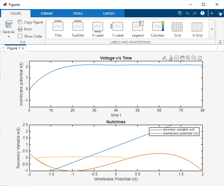
The FitzHugh–Nagumo model was simulated in MATLAB and Proteus to analyze neuronal excitability. In MATLAB, the system of nonlinear differential equations was solved using the ODE45 solver for different parameter sets and input stimuli. The time-domain plots of the membrane potential clearly showed threshold-dependent firing. For subthreshold inputs, the system stabilized at a resting potential, while for suprathreshold inputs, full action potential spikes were generated. The recovery variable exhibited slower dynamics, confirming its role in controlling the refractory phase. Phase-plane trajectories illustrated the existence of limit cycles under continuous excitation, demonstrating oscillatory firing behavior. Parameter sensitivity analysis showed that variations in ε and input current significantly affected spike frequency and stability.

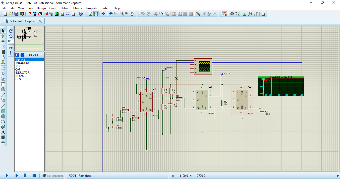
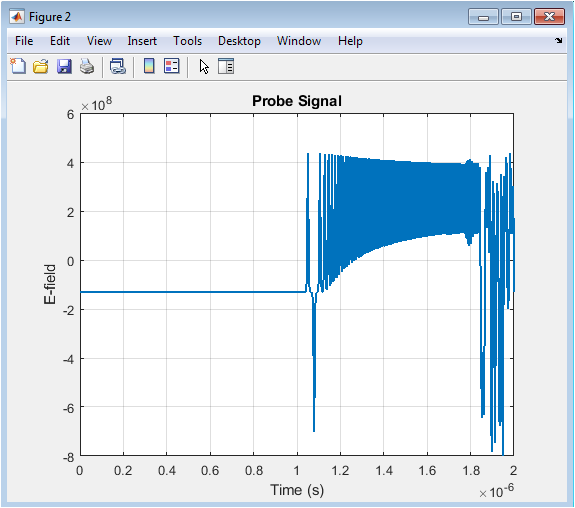
In Proteus, the electronic circuit equivalent of the FitzHugh–Nagumo model was designed using operational amplifiers, resistors, capacitors, and diodes. A nonlinear amplifier configuration was employed to replicate the cubic nonlinearity present in the mathematical model. When a current source stimulus was applied, the circuit produced voltage waveforms resembling action potentials. The output confirmed excitability: below a threshold, the circuit remained inactive, while above threshold, it produced repetitive spiking. The simulated waveforms closely matched those from MATLAB, validating the equivalence between the mathematical and hardware implementations.

You can download the Project files here: Download files now. (You must be logged in).

Comparative analysis between MATLAB and Proteus simulations demonstrated strong consistency. Both environments captured the essential characteristics of neuronal excitability, including threshold behavior, spike generation, refractory dynamics, and oscillations. The Proteus hardware model provided additional insights into practical realizations of neuromorphic circuits, confirming that the FitzHugh–Nagumo model can be effectively applied to analog circuit design for neuroscience and biomedical applications.

7- Conclusion

This project successfully demonstrated the design, simulation, and analysis of the FitzHugh–Nagumo model for neuronal excitability using both MATLAB and Proteus. The MATLAB implementation provided numerical insights into the temporal and phase-plane dynamics of neuron-like firing, while the Proteus circuit design validated the model in a hardware-equivalent analog form. Results confirmed that the model exhibits threshold-dependent excitability, action potential generation, and oscillatory behavior consistent with biological neurons. The dual approach ensured not only mathematical accuracy but also practical feasibility, making the model highly suitable for applications in neuromorphic hardware, neural prosthetics, and educational demonstrations. The work highlights the effectiveness of simplified neuronal models in bridging the gap between theoretical neuroscience and real-world engineering systems.

8- References

1. FitzHugh, R. (1961). Impulses and physiological states in theoretical models of nerve membrane. Biophysical Journal, 1(6), 445–466.
2. Nagumo, J., Arimoto, S., & Yoshizawa, S. (1962). An active pulse transmission line simulating nerve axon. Proceedings of the IRE, 50(10), 2061–2070.
3. Hodgkin, A. L., & Huxley, A. F. (1952). A quantitative description of membrane current and its application to conduction and excitation in nerve. Journal of Physiology, 117(4), 500–544.
4. Izhikevich, E. M. (2007). Dynamical Systems in Neuroscience: The Geometry of Excitability and Bursting. MIT Press.
5. Keener, J., & Sneyd, J. (2009). Mathematical Physiology. Springer.
6. Koch, C. (1999). Biophysics of Computation: Information Processing in Single Neurons. Oxford University Press.
7. Ermentrout, G. B., & Terman, D. H. (2010). Mathematical Foundations of Neuroscience. Springer.
8. Dayan, P., & Abbott, L. F. (2001). Theoretical Neuroscience: Computational and Mathematical Modeling of Neural Systems. MIT Press.
9. Rinzel, J., & Ermentrout, G. B. (1998). Analysis of neural excitability and oscillations. Methods in Neuronal Modeling, MIT Press.
10. Chua, L. O., & Roska, T. (2002). Cellular Neural Networks and Visual Computing: Foundations and Applications. Cambridge University Press.
11. Steven H. Strogatz, Nonlinear Dynamics and Chaos with Applications to Physics, Biology, Chemistry and Enigneering
12. FitzHugh R. (1961) Impulses and physiological states in theoretical models of nerve membrane. Biophysical J. 1:445-466
13. Nagumo J., Arimoto S., and Yoshizawa S. (1962) An active pulse transmis- sion line simulating nerve axon. Proc IRE. 50:2061–2070.
14. D.Murray, Mathematical Biology: I. An introduction, third edition

You can download the Project files here: Download files now. (You must be logged in).

Keywords: FitzHugh–Nagumo model, neuronal excitability, action potential simulation, MATLAB differential equations, Proteus circuit design, phase plane analysis, nonlinear dynamics, neuronal spiking behavior, bioelectronic modeling, computational neuroscience.

Do you need help with Circuit design and Proteus Simulation based projects? Don’t hesitate to contact our Tutors to receive professional and reliable guidance.