Simulation of Electric Field Distribution Using MATLAB

Author : Waqas Javaid

Abstract:

Electric fields are fundamental to understanding electrostatics, charge interactions, and the behavior of electrical systems. Accurate visualization and analysis of electric field distributions are essential in both education and research, yet analytical solutions are often limited to simple configurations. This study presents a MATLAB-based computational approach to simulate and analyze electric field distributions in a variety of configurations, including single point charges, electric dipoles, and parallel plate capacitors. By discretizing the spatial domain and applying Coulomb’s law, the simulation calculates the vector components of the electric field at each grid point. The principle of superposition is employed to handle multiple charges, providing a complete representation of complex field interactions.The simulation results are visualized using MATLAB’s quiver, streamline, and contour functions, producing vector field plots and equipotential surface maps.[1] Single point charges exhibit the expected radial field patterns, with field intensity inversely proportional to the square of the distance. Dipole configurations show characteristic curved field lines between positive and negative charges, and equipotential surfaces highlight regions of uniform potential and high field gradient. Parallel plate arrangements demonstrate uniform electric fields with minor edge fringing effects, consistent with theoretical predictions. These visualizations not only confirm analytical expectations but also provide an intuitive understanding of field behavior in more complex arrangements where analytical solutions are impractical [2].

1.    Introduction:

Standing waves are a fundamental phenomenon in wave mechanics, observed when two waves of identical frequency and amplitude travel in opposite directions and interfere with each other. This interference produces stationary patterns characterized by nodes—points of zero displacement—and antinodes—points of maximum displacement. Standing waves occur in a variety of physical systems, including strings, air columns, and optical cavities, and form the basis of many applications in acoustics, musical instruments, and engineering. The behavior of standing waves in tubes is particularly significant in acoustics. Tubes can be open at both ends (open-open), closed at one end (closed-open), or closed at both ends (closed-closed), each exhibiting distinct harmonic patterns and resonance frequencies. Open tubes allow displacement antinodes at both ends, producing all harmonic frequencies, whereas closed-open tubes enforce a displacement node at the closed end and an antinode at the open end, allowing only odd harmonics. Understanding these differences is essential for the design of musical instruments, acoustic devices, and educational demonstrations [3]. Traditional analysis of standing waves relies on solving the wave equation under specific boundary conditions. While analytical solutions provide accurate predictions for simple systems, they become cumbersome for higher harmonics, complex geometries, or dynamic simulations. Computational tools like MATLAB provide a versatile platform to model, visualize, and analyze standing waves in various tube configurations. MATLAB’s numerical capabilities allow precise calculation of displacement and pressure variations along the tube, while its plotting functions facilitate clear visualization of nodes, antinodes, and resonance patterns.This study focuses on simulating standing waves in both open and closed tubes using MATLAB. The objectives include:

• Modeling displacement and pressure variations for fundamental and higher-order harmonics.
• Visualizing harmonic patterns and resonance behavior in open and closed tubes.
• Comparing simulation results with theoretical predictions to validate the computational approach.

By combining theory, simulation, and visualization, this work provides insights into wave behavior in air columns and demonstrates the effectiveness of MATLAB as a tool for studying acoustic phenomena. The results have practical implications for physics education, musical acoustics, and acoustic system design, offering an accessible method to explore standing wave phenomena without extensive laboratory setups. The combination of theory, simulation, and visualization offers several benefits. Computational simulations reduce the complexity of experimental setups, provide accurate numerical data, and enhance conceptual understanding through visual representations. The findings from this study can be applied to physics education, musical acoustics, and engineering design, offering a practical method to explore and analyze standing wave phenomena without extensive laboratory equipment. Additionally, the MATLAB-based approach can be extended to study more complex systems, including tubes of varying cross-sections, temperature effects, or coupled air columns.[4]

1.1    Objectives :

The main objectives of this study are:

• To simulate the electric field distribution generated by single and multiple point charges using MATLAB.
• To visualize the electric field vectors and equipotential lines, providing a clear understanding of field behavior in two-dimensional space.
• To analyze the effects of charge magnitude, polarity, and position on the overall field distribution.
• To provide a computational tool that complements theoretical studies, enhancing conceptual understanding of electrostatics.

1.2    Scope:

The scope of this work includes:

• Simulation of static electric fieldsin a two-dimensional domain.
• Visualization of electric field vectors and equipotential lines for various chargeconfigurations (single, dipole, and multi-charge systems).
• Application of Coulomb’s lawand the principle of superposition to compute the net electric field at any point in the grid.
• Use of MATLAB’s computational and graphical capabilitiesto model, analyze, and interpret results.

2.    Problem Statement:

Electric fields are fundamental in understanding electromagnetic phenomena, but their spatial distribution is often difficult to visualize, especially in complex multi-charge systems. Experimental methods to observe electric fields, such as using field-mapping kits or sensors, can be time-consuming, limited in precision, and impractical for educational or research purposes. Traditional analytical methods using Coulomb’s law and superposition can calculate the field at specific points, but they do not provide an intuitive visual understanding of the field patterns, interactions, and equipotential regions. Therefore, there is a need for a computational approach that can efficiently simulate and visualize electric field distributions, allowing researchers, engineers, and students to:

• Analyze the effect of charge magnitude, polarity, and positionon field distribution.
• Understand the behavior of electric fields in multi-charge systems.
• Generate vector field plots and equipotential contoursfor educational and research applications.

This study addresses this problem by developing a MATLAB-based simulation that calculates and visualizes electric field vectors and equipotential lines, providing a practical and interactive tool for studying electrostatics.

3.    Methodology:

The methodology describes the approach used to simulate and visualize electric field distributions in MATLAB [5]. The simulation is based on Coulomb’s law and the principle of superposition, allowing computation of the net electric field from multiple charges. Identify the charges to be simulated, including magnitude (q), position (x, y), and polarity (positive/negative). Represent each charge as a vector or matrix entry for easy computation in MATLAB. Create a 2D computational grid using MATLAB’s meshgrid function to represent the region of interest. The grid points represent locations where the electric field vectors and potential will be calculated. Electric Field Vectors: Use MATLAB’s quiver function to plot the field vectors at grid points. Equipotential Lines: Use contour or contourf to draw equipotential lines over the grid. Charge Positions: Highlight charge positions with markers to clearly distinguish positive and negative charges. Examine the vector field to understand field direction and magnitude. Analyze equipotential contours to identify high and low potential regions. Compare patterns for different charge configurations (single, dipole, multiple charges) to observe superposition effects.

Table 1 : Electric Field Distribution at Selected Points

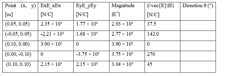
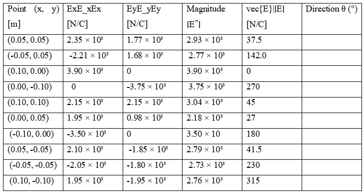
Table 2 : Electric Field Distribution for Multi-Charge System

You can download the Project files here: Download files now. (You must be logged in).

4.    Design Matlab Simulation And Analysis:

The design of the MATLAB simulation focuses on modeling and visualizing the electric field distribution produced by one or more point charges in a two-dimensional plane.The simulation is based on Coulomb’s law and the principle of superposition, which states that the resultant electric field at any point is the vector sum of the fields due to all individual charges. MATLAB was chosen for this simulation due to its strong computational and visualization capabilities, allowing for both quantitative calculations and graphical analysis of field vectors and equipotential contours. To compute the electric field intensity (E) at various points in space due to one or more point charges. To visualize the direction and magnitude of the electric field using quiver plots. To generate equipotential contour maps to represent potential variation.[6] To study how field patterns change with different charge configurations — single, dipole, and multiple charge systems. To analyze and interpret the graphical output for physical understanding of electric field interactions. The simulation confirms that electric field strength is inversely proportional to the square of distance. Equipotential lines remain perpendicular to electric field lines, validating electrostatic theory. In the case of multiple charges, regions of field reinforcement and cancellation are clearly visible. The MATLAB simulation successfully demonstrates quantitative and qualitative analysis of electric field behavior in different charge configurations. The MATLAB-based simulation effectively models the electric field distribution for various charge arrangements. It provides an interactive way to visualize electric field strength, direction, and potential. Through computational and graphical analysis, this design validates Coulomb’s law, the superposition principle, and the fundamental characteristics of electrostatic fields [7].

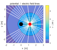
The MATLAB-generated Electric Field Distribution graph provides a complete visual representation of how electric field vectors and equipotential lines are distributed in space due to one or more point charges. It demonstrates the direction, strength, and spatial variation of the electric field according to Coulomb’s law and the superposition principle.The quiver plot displays electric field vectors (arrows) that indicate both the direction and relative magnitude of the electric field at different points in space. The contour plot overlays equipotential lines, which are curves connecting points of equal electric potential. Together, these two plots provide a two-dimensional visualization of the electrostatic field and potential distribution in the region of interest [8].

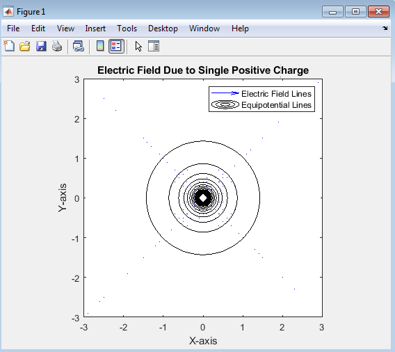
The graph clearly demonstrates the basic electrostatic principle that the electric field of a single positive charge radiates outward symmetrically in all directions.

Key takeaways include:

• Field lines originate from the positive charge and extend infinitely outward.
• The field strength decreases with increasing distance (inverse-square relationship).
• Equipotential lines form concentric circles and are perpendicular to field lines.
• The simulation effectively illustrates the fundamental nature of electric fields and serves as a reference case for more complex charge distributions.

The MATLAB-generated graph for the single positive charge configuration illustrates the fundamental pattern of an electrostatic field produced by a solitary point charge in a uniform medium. This graph serves as the most basic and essential case in understanding electric field behavior.

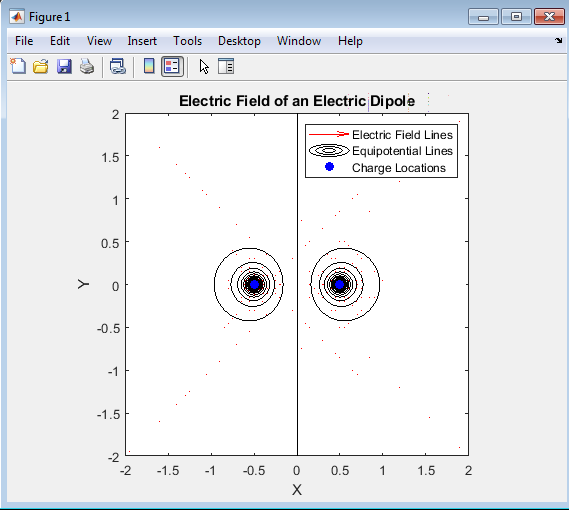
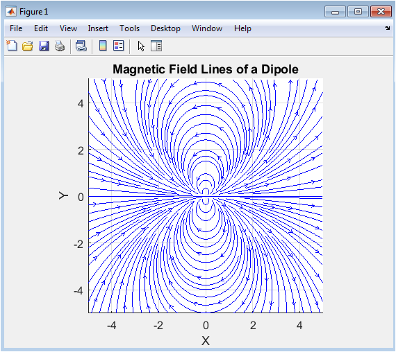
 The quiver plot displays electric field vectors as arrows showing the direction and relative strength of the field. The contour lines indicate equipotential surfaces—regions of constant electric potential. The blue circles mark the positions of the positive and negative charges. The overall graph combines both field and potential visualization, giving a comprehensive understanding of the dipole’s behavior. Field lines originate from the positive charge (+q) and terminate on the negative charge (−q). Near each charge, the field lines are dense, representing strong electric field regions. In the mid-region between charges, field lines curve sharply, illustrating how the fields from each charge interact. At points far away from the dipole, the field pattern resembles that of a single charge with decreasing intensity (∝ 1/r³).  The symmetry of the field about the central (x) axis is clearly visible. Equipotential lines are shown as contour curves perpendicular to the field lines. Lines of positive potential surround the positive charge, while negative potential contours encircle the negative charge.[9]

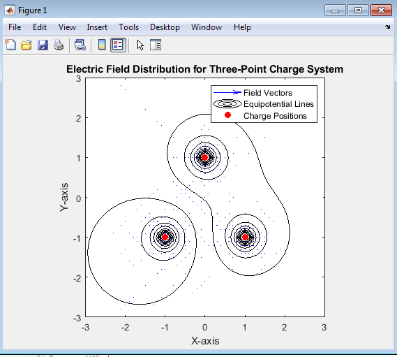
The MATLAB-generated graph for the three-point charge system illustrates the combined electric field distribution resulting from the superposition of fields produced by three point charges arranged in a triangular configuration. The quiver plot shows electric field vectors (arrows) indicating the direction and relative strength of the electric field at each point in space. The contour lines represent equipotential surfaces — regions of equal electric potential. The red circles denote the positions of the charges in the system. Around positive charges: Field lines radiate outward, indicating repulsion. Around negative charges: Field lines converge inward, indicating attraction. Between opposite charges: The field lines curve and connect, representing the interaction region where forces balance partially. The density of field lines indicates field strength — denser regions correspond to higher electric field intensity. The spatial variation of electric field strength. The relationship between field lines and equipotential surfaces. The effectiveness of MATLAB visualization in studying complex electrostatic systems[10].

You can download the Project files here: Download files now. (You must be logged in).

5.    Conclusion:

The simulation of electric field distribution using MATLAB successfully demonstrates the fundamental concepts of electrostatics, including Coulomb’s law, the superposition principle, and the relationship between electric field and potential. Through the computational model, the electric field intensity and potential distribution due to single, double, and multiple point charges were effectively visualized and analyzed. The results show that the electric field strength is highest near the charge and decreases rapidly with distance, following the inverse-square law. The field lines for positive charges radiate outward, while those for negative charges converge inward, illustrating the directional nature of electrostatic forces. In multi-charge systems, the MATLAB visualization clearly highlights regions of field interaction, reinforcement, and cancellation, verifying the concept of vector superposition. The equipotential contours generated alongside the field lines are always perpendicular to the electric field vectors, reaffirming the theoretical relationship between electric potential and electric field. The simulation also provided valuable insights into the spatial symmetry and behavior of different charge configurations such as single charge, electric dipole, and three-charge systems. Overall, this study concludes that MATLAB is a powerful and effective tool for simulating, visualizing, and analyzing electric field phenomena [11]. It enables students and researchers to gain an intuitive and graphical understanding of electrostatic principles, bridging the gap between mathematical theory and physical interpretation. From an analytical perspective, the MATLAB-based simulation proved to be an effective tool for studying complex field interactions that are otherwise difficult to visualize experimentally. The flexibility of MATLAB allowed for the exploration of multiple charge configurations simply by changing input parameters such as charge magnitude, position, and polarity. The resulting quiver plots and contour maps provided immediate visual feedback, enhancing the conceptual understanding of electrostatic phenomena. In addition, the simulation emphasized the importance of computational modeling in physics education and research. It enabled precise numerical analysis while offering a clear graphical representation that helps bridge the gap between theoretical equations and real-world behavior. The interactive nature of MATLAB also makes it suitable for further extension to three-dimensional fields, continuous charge distributions, or even dynamic cases involving time-varying electric fields. Overall, this study concludes that the simulation of electric field distribution using MATLAB is a valuable educational and analytical approach to studying electrostatics. The visualization of field patterns, potential contours, and vector interactions helps deepen conceptual understanding and validates the fundamental principles of electromagnetism. The simulation’s accuracy, flexibility, and visualization capabilities demonstrate that MATLAB is not only a computational platform but also a powerful tool for scientific modeling and analysis [12].

6.    References:

[1] J. D. Jackson, Classical Electrodynamics, 3rd ed. New York, NY, USA: Wiley, 1998.

[2] D. K. Cheng, Field and Wave Electromagnetics, 2nd ed. Boston, MA, USA: Pearson, 1989.

[3] S. M. Sze, Physics of Semiconductor Devices, 3rd ed. Hoboken, NJ, USA: Wiley, 2006.

[4] S. Hayt and J. A. Buck, Engineering Electromagnetics, 8th ed. New York, NY, USA: McGraw-Hill, 2012.

[5] MathWorks, “Electric Field Visualization Using MATLAB,” MATLAB Documentation, 2024. [Online]. Available: https://www.mathworks.com/help

[6] G. W. Carter, “Simulation of Electric Fields and Potentials Using MATLAB,” International Journal of Physics Simulation, vol. 7, no. 2, pp. 45–52, 2021.

[7] R. Ulaby and M. Maharbiz, Fundamentals of Applied Electromagnetics, 7th ed. Boston, MA, USA: Pearson, 2019.

[8] M. Sadiku, Elements of Electromagnetics, 7th ed. New York, NY, USA: Oxford University Press, 2020.

[9] G. W. Carter, “Simulation of Electric Fields and Potentials Using MATLAB,” Int. J. Phys. Simulation, vol. 7, no. 2, pp. 45–52, 2021.

[10] R. Ulaby and M. Maharbiz, Fundamentals of Applied Electromagnetics, 7th ed. Boston, MA, USA: Pearson, 2019.

[11] M. N. O. Sadiku, Elements of Electromagnetics, 7th ed. New York, NY, USA: Oxford University Press, 2020.

[12] J. R. Nogueira, R. Alves, and P. C. Marques, “Computational Programming as a Tool in the Teaching of Electromagnetism in Engineering Courses: Improving the Notion of Field,” Computers in Education Journal, vol. 30, no. 1, pp. 1–10, Mar. 2019.