

Next Generation Benchmark Framework for Structural Control of Seismically Excited High-Rise Buildings
Author: Waqas Javaid
Abstract
This paper presents the problem definition and guidelines of the next generation structural control benchmark problem for seismically excited buildings. Focusing on a 20-story steel struc- ture representing a typical mid- to high-rise building designed for the Los Angeles, California region, the goal of this study is to provide a clear basis to evaluate the efficacy of various struc- tural control strategies. An evaluation model has been developed that portrays the salient features of the structural system. Control constraints and evaluation criteria are presented for the design problem. The task of each participant in this benchmark study is to define (including devices, sen- sors and control algorithms), evaluate and report on their proposed control strategies. These strat- egies may be either passive, active, semi-active or a combination thereof. A simulation program has been developed and made available to facilitate direct comparison of the efficiency and merit of the various control strategies. To illustrate some of the design challenges a sample control sys- tem design is presented, although this sample is not intended to be viewed as a competitive design.
Introduction
The protection of civil structures, including material content and human occupants, is with- out a doubt a world-wide priority. The extent of protection may range from reliable operation and occupant comfort to human and structural survivability. Civil structures, including existing and future buildings, towers and bridges, must be adequately protected from a variety of events, including earthquakes, winds, waves and traffic. The protection of structures is now moving from relying entirely on the inelastic deformation of the structure to dissipate the energy of severe dynamic loadings, to the application of passive, active and semi-active structural control devices to mitigate undesired responses to dynamic loads.
In the last two decades, many control algorithms and devices have been proposed for civil engineering applications (Soong 1990; Housner, et al. 1994; Soong and Constantinou 1994; Fujino, et al. 1996; Spencer and Sain 1997), each of which has certain advantages, depending on the specific application and the desired objectives. At the present time, structural control research is greatly diversified with regard to these specific applications and desired objectives. A common basis for comparison of the various algorithms and devices does not currently exist. Determination of the general effectiveness of structural control algorithms and devices, a task which is necessary to focus future structural control research and development, is challenging.
Ideally, each proposed control strategy should be evaluated experimentally under conditions that closely model the as-built environment. However, it is impractical, both financially and logis- tically, for all researchers in structural control to conduct even small-scale experimental tests. An available alternative is the use of consensus-approved, high-fidelity, analytical benchmark models to allow researchers in structural control to test their algorithms and devices and to directly com- pare the results.
The American Society of Civil Engineers (ASCE) Committee on Structural Control has rec- ognized the significance of structural control benchmark problems. The Committee recently developed a benchmark study, focusing primarily on the comparison of structural control algo- rithms for three-story building models. The initial results of this study were reported at the 1997 ASCE Structures Congress, held in Portland, Oregon (Spencer, et al. 1997; Balas, 1997; Lu and Skelton 1997; Wu, et al. 1997; Smith, et al. 1997). Additionally, a more extensive analysis of the benchmark structural control problem is nearing completion and will form the basis for a special issue of Earthquake Engineering and Structural Dynamics (Spencer, et al. 1998).
Building on the foundation laid by the ASCE Committee on Structural Control, plans for the next generation of benchmark structural control studies were initiated by the Working Group on Building Control during the Second International Workshop on Structural Control held December 18–20, 1996, in Hong Kong (Chen 1996). As stated by the Working Group, the goal of this effort is to develop benchmark models to provide systematic and standardized means by which competing control strategies, including devices, algorithms, sensors, etc., can be evaluated. This goal drives the next generation of structural control benchmark problems, and its achieve- ment will take the structural control community another step toward the realization and imple- mentation of innovative control strategies for dynamic hazard mitigation [2] [3].
As an outgrowth of the workshop in Hong Kong, two benchmark problems for the control of buildings have been developed for presentation at the 2nd World Conference on Structural Control to be held June 28–July 1, 1998 in Kyoto, Japan. The first, detailed in Yang, et al. (1998), proposes a benchmark problem for wind excited buildings. The second such benchmark problem is defined herein, the focus of which is to provide the guidelines for the next generation bench- mark control problem for seismically excited buildings. A 20-story steel building designed for the SAC4 project is the benchmark structure to be studied. A description of this structure is discussed in the next section. A high-fidelity linear time-invariant state space model of this structure was developed and is designated the evaluation model. In the context of this study, the evaluation model is considered to be a true model of the structural system. Several evaluation criteria, mea- suring the effectiveness of the control strategy to reduce undesired responses of the evaluation model to ground excitation, are given, along with the associated control design constraints.
Designers/researchers participating in this benchmark study shall define (including devices, sen- sors and control algorithms), evaluate and report the results for their proposed control strategies. The location on the structure and an appropriate model must be specified for each control device and sensor employed. Passive, active and semi-active devices, or a combination thereof, may be considered. For illustrative purposes a complete sample control design is presented. Although this sample control system it not intended to be competitive, it demonstrates how one might define and model the sensors and control devices employed, build a design model, and evaluate a complete control system design.
Benchmark Structure
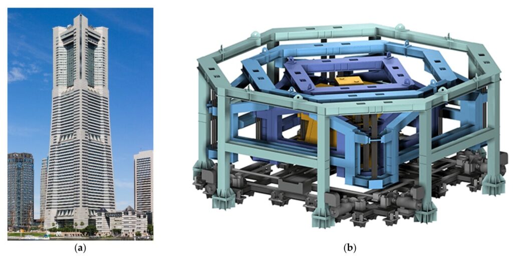
The 20-story structure used for this benchmark study was designed by Brandow & Johnston Associates5 for the SAC Phase II Steel Project. Although not actually constructed, the structure meets seismic code and represents a typical mid- to high-rise building designed for the Los Ange- les, California region. This building was chosen because it will also serve as a benchmark struc- ture for SAC studies and thus will provide a wider basis for comparison of the results from the present study.
The Los Angeles twenty-story (LA 20-story) structure is 30.48 m (100 ft) by 36.58 m (120 ft) in plan, and 80.77 m (265 ft) in elevation. The bays are 6.10 m (20 ft) on center, in both direc- tions, with five bays in the north-south (N-S) direction and six bays in the east-west (E-W) direc- tion. The building’s lateral load-resisting system is comprised of steel perimeter moment-resisting frames (MRFs). The interior bays of the structure contain simple framing with composite floors.
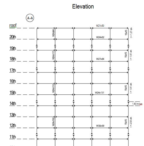
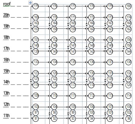
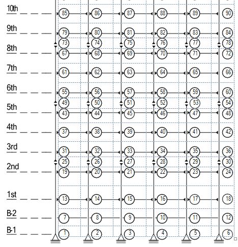
The columns are 345 Mpa (50 ksi) steel. The interior columns of the MRF are wide-flange. The corner columns are box columns. The levels of the 20-story building are numbered with respect to the first story, located at the ground (first) level (see Fig. 1). The 21st level is denoted the roof. The building has an additional two basement levels. The level directly below the ground level is the second basement (B-2). The level below B-2 is the first basement (B-1). Typical floor- to-floor heights (for analysis purposes measured from center-of-beam to center-of-beam) are 3.96 m (13 ft). The floor-to-floor heights for the two basement levels are 3.65 m (12 ft) and for the first floor is 5.49 m (18 ft) [1].
The column lines employ three-tier construction, i.e. monolithic column pieces are con- nected every three levels beginning with the second story. Column splices, which are seismic (ten- sion) splices to carry bending and uplift forces, are located on the 2nd, 5th, 8th, 11th, 14th, 17th and 19th stories at 1.83 m (6 ft) above the center-line of the beam to column joint. The column bases are modeled as pinned (at the B-1 level) and secured to the ground. Concrete foundation walls and surrounding soil are assumed to restrain the structure at the first floor from horizontal displacement.
The floors are composite construction (i.e., concrete and steel). In accordance with common practice, the floor system, which provides diaphragm action, is assumed to be rigid in the horizon-
tal plane. The floor system is comprised of 248 Mpa (36 ksi) steel wide-flange beams acting com- positely with the floor slab. The B-2 floor beams are simply connected to the columns. The inertial effects of each level are assumed to be carried evenly by the floor diaphragm to each perimeter MRF, hence each frame resists one half of the seismic mass associated with the entire structure.
The seismic mass of the structure is due to various components of the structure, including the steel framing, floor slabs, ceiling/flooring, mechanical/electrical, partitions, roofing and a penthouse located on the roof. The seismic mass of the first level is 5.32×10⁵ kg (36.4 kips-sec2/ ft), for the second level is 5.65×10⁵ kg (38.7 kips-sec2/ft), for the third level to 20th level is
5.51×10⁵ kg (37.7 kips-sec2/ft), and for the roof is 5.83×10⁵ kg (39.9 kips-sec2/ft). The seismic mass of the entire structure is 1.16×10⁷ kg (794 kips-sec2/ft).
This benchmark study will focus on an in-plane (2-D) analysis of one-half of the entire structure. The frame being considered in this study is one of the N-S MRFs (the short direction of the building). The height to width ratio for the N-S frame is 2.65:1. The N-S MRF is depicted in Fig. 1.
Passive, active and/or semi-active control devices can be implemented throughout the N-S frame of the 20-story structure and their performance assessed using the evaluation models speci- fied in the next section.
Evaluation Model
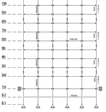
Based on the physical description of the LA 20-story structure described in the previous section, an in-plane finite element model of the N-S MRF is developed in MATLAB (1997). Because the focus of this study is on global response characteristics, considering the linearized response of the structure can be shown to be a reasonable approximation (Naeim 1997) that will be used for the purposes of this study. The structure is modeled as a system of plane-frame ele- ments, and mass and stiffness matrices for the structure are determined. Due to the size of the model, a Guyan reduction is used to reduce the number of DOFs to a manageable size, while still maintaining the important dynamics of the full model [1] [2]. Using the reduced mass and stiffness matrices, the damping matrix is determined based on an assumption of modal damping. The equa- tions of motion for the structure are then developed in a state space form appropriate for design and analysis. This process, described in further detail in the following paragraphs, is illustrated in Fig. 2.
The LA 20-story structure is modeled using 180 nodes interconnected by 284 elements, as seen in Fig. 3. The nodes are located at beam-to-column joints and at column splice locations. Elements are created between nodes to represent the beams and columns in the structure. The beam members extend from the center-line of column to center-line of column, thus ignoring the column panel zone [3]. Floor inertial loads, accounting for the seismic mass of the floor slabs, ceil- ing/flooring, mechanical/electrical, partitions, roofing and penthouse are uniformly distributed at the nodes of each respective floor assuming a consistent mass formulation.
You can download the Project files here: Download files now. (You must be logged in).
Each node has three degrees-of-freedom (DOFs): horizontal, vertical and rotational. The entire structure has 540 DOFs prior to application of boundary conditions/constraints and subse-
quent model reduction. Global DOF n is the jth local DOF (i.e., horizontal: j = 1, vertical: j = 2,
rotation: j = 3) of the ith node as given by n = 3(i – 1) + j .
The evaluation model focuses on one of the two N-S MRFs of the LA-20 story structure. This single N-S frame is assumed to support one half of the seismic mass of the entire structure (i.e., 2.66×10⁵ kg (18.2 kips-sec2/ft) for the first level, 2.83×10⁵ kg (19.4 kips-sec2/ft) for the sec- ond level, 2.76×10⁵ kg (18.9 kips-sec2/ft) for the third to 20th levels, and 2.92×10⁵ kg (20.0 kips- sec2/ft) for the roof). Additionally, for modeling purposes, the seismic mass is broken into two components: the steel framing, including beams and columns, and all other additional seismic mass. The seismic mass of the steel framing of a single N-S MRF is 2.64×10⁵ kg (18.1 kips-sec2/ ft). The seismic mass of a single N-S MRF, without the mass of the steel framing, for the first level is 2.54×10⁵ kg (17.4 kips-sec2/ft), for the second level is 2.70×10⁵ kg (18.5 kips-sec2/ft), for the third level to 20th level is 2.63×10⁵ kg (18.0 kips-sec2/ft) and for the roof is 2.79×10⁵ kg (19.1 kips-sec2/ft). The seismic mass of the N-S MRF is 5.80×10⁶ kg (397 kips-sec2/ft). The seismic mass of all above ground floors of the N-S MRF, neglecting the mass of the first level, is 5.543×10⁶ kg (379 kips-sec2/ft) [4] [5].
Each element, modeled as a plane frame element, contains two nodes and six DOFs. The length, area, moment of inertia, modulus of elasticity and mass density are pre-defined for each element. The elemental consistent mass and stiffness matrices are determined as functions of these properties (Sack 1989; Cook, et. al 1989).
Global mass and stiffness matrices are assembled from the elemental mass and stiffness matrices by summing the mass and stiffness associated with each DOF for each element of the entire structure. The DOFs corresponding to fixed boundary conditions are then constrained by eliminating the rows and columns associated with these DOFs from the global mass and stiffness matrices [6] [7]. The constrained DOFs are the horizontal DOFs at nodes 1, 2, 3, 4, 5, 6, 13 and 18 and
the vertical DOFs at nodes 1, 2, 3, 4, 5 and 6. Realizing these 14 boundary conditions results in
the mass matrix, M [526 ´ 526 ], and the stiffness matrix, K [526 ´ 526 ]. The equation of motion for the undamped structural system takes the form
![]()
where U˙˙ is the second time derivative of the response vector U , x˙˙g (m/sec2) is the ground acceleration, f (kN) is the control force input, G is a vector of zeros and ones defining the loading of the ground acceleration to the structure, and P is a vector defining how the force(s) produced by the control device(s) enter the structure. Responses for a particular level are measured at the floor of the level in question. The horizontal responses are relative to the ground.
Because the floor slab is assumed to be rigid in its horizontal plane, the nodes associated with each floor have the same horizontal displacements. This assumption is enforced by writing constraint equations relating the dependent (slave) horizontal DOFs on each floor slab to a single active horizontal DOF and using a Ritz transformation (Craig, 1981). First, the structural responses are partitioned in terms of active and dependent DOFs as U = [UT UT]T, and the constraint equations are written in the form RdaUa + RddUd = 0 . The mass and stiffness matrices are similarly partitioned in terms of active and dependent DOFs
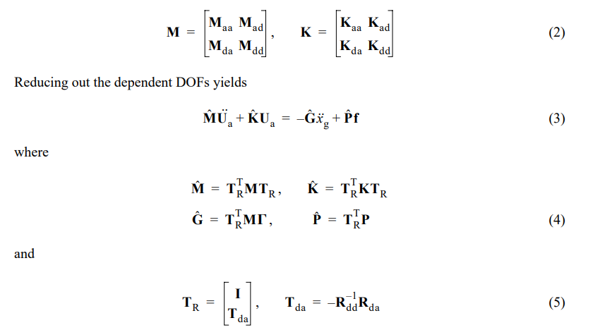
I is an appropriately sized identity matrix. Note that G and P also must be reordered correspond- ing to the active and dependent DOFs prior to making the transformation in Eq. (4). The number of DOFs in the resulting model is 418.
The next step in forming the evaluation model is model reduction. A model with 418 DOFs is computationally burdensome for dynamic analysis. The natural frequencies of the higher modes in this model are excessively large. As these modes, attributed mostly to rotational and vertical DOFs, are unlikely to contribute to the response of the physical system, they are not required for the benchmark model and can be reduced out. A Guyan reduction (Craig 1981) of all of the rota- tional and most of the vertical DOFs is used to reduce the 418 DOF model to nearly 1/5 of its original size [8] [9].
Again, the DOFs are partitioned into active and dependent (slave) DOFs. The active hori- zontal DOFs, as well as the vertical DOFs for levels 1–21 located on the second and fifth column lines, are chosen to be active. All other vertical DOFs, including the vertical DOFs at splice loca- tions, and all rotational DOFs are assumed dependent and condensed out. The mass and stiffness matrices are partitioned in terms of the active and dependent degrees of freedom, i.e.,
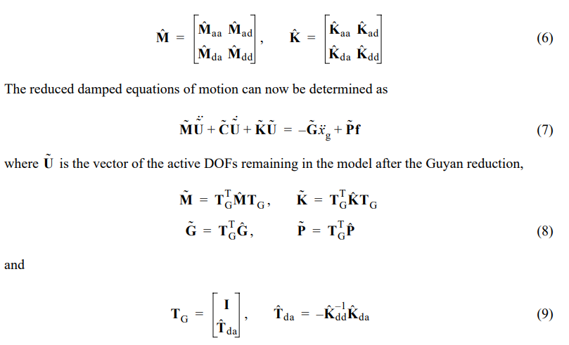
Again, Gˆ and Pˆ are reordered corresponding to the active and dependent DOFs prior to making the transformation in Eq. (8).
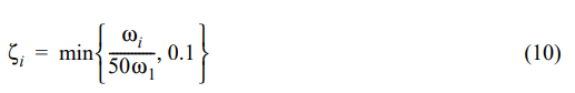
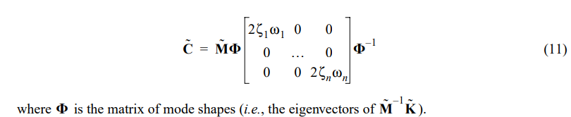
The damping matrix C˜ is defined based on the reduced system and the assumption of modal damping. Damping in each mode is assumed to be proportional to the mode’s associated frequency, with a maximum of 10% critical damping in any one mode. The damping in the first mode is assumed to be 2%; therefore the damping zi in the ith mode is given by
The Guyan reduction results in a final model with 106 DOFs, that maintains the important dynamics of the original model. The natural frequencies of the resulting model are less than 110 Hz [10].
A state space representation of the input-output model for the LA 20-story structure is now developed. The model is of the form
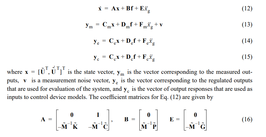
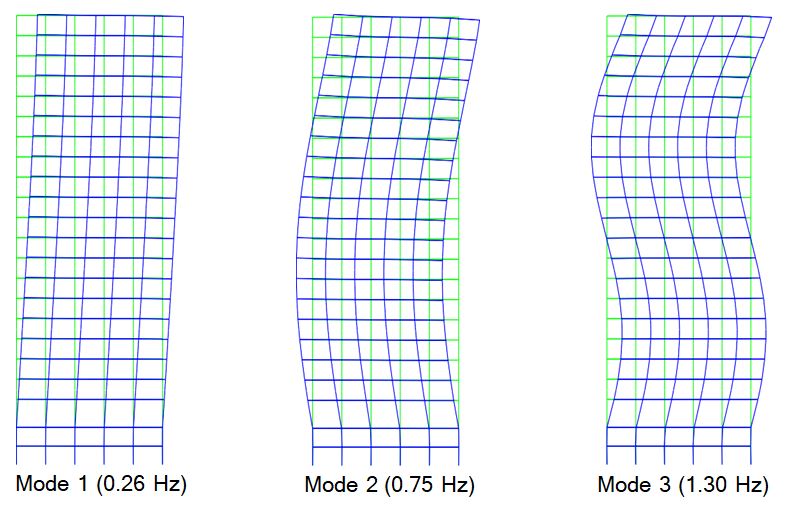
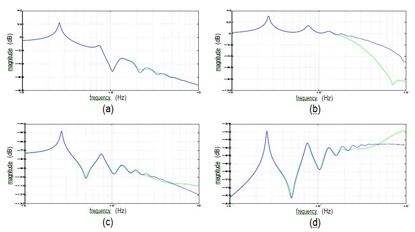
The model of Eqs. (12–15) represents the input-output behavior of the LA 20-story struc- ture considered for this study. The first 10 natural frequencies of this model are: 0.26, 0.75, 1.30, 1.83, 2.40, 2.80, 3.00, 3.21, 3.63 and 4.31 Hz. These results are consistent with those found by others who have modeled this structure. The first three mode shapes are given in Fig 4. Typical transfer functions for this structure comparing the reduced and full models are given in Fig. 5.
You can download the Project files here: Download files now. (You must be logged in).
Degradation Effects
The change of the dynamic properties of a building from before (pre-earthquake) to after (post-earthquake) a strong motion earthquake can be substantial (Naeim 1997). This change can
cause as much as a 20% increase in the fundamental period, which is primarily due to stiffness degradation. Such stiffness reduction is attributed to the loss of non-structural elements and to damage of structural elements. Because the time between the main earthquake and subsequent significant aftershocks may not be large, an effective control system should be sufficiently robust to perform adequately based either on the pre-earthquake structure or the post-earthquake struc- ture [11].
Two evaluation models are developed from the previously defined nominal structural model: the pre-earthquake evaluation model and the post-earthquake evaluation model. These two models are intended to account for the degradation effects that can occur within the structure dur- ing a strong ground motion and should be viewed as linearized models of the structure before and after degradation of the structure has occurred. The degradation of the benchmark building is modeled as a reduction in stiffness from the pre-earthquake to post-earthquake models. It should be noted that the post-earthquake building model assumes structural damage has occurred, which may be potentially avoided through the application of control device(s). Therefore, the post-earth- quake building model may be viewed in some sense as representing a “worst-case” scenario.
The pre-earthquake evaluation model represents the LA 20-story structure as-built. The as- built structure includes additional stiffness provided by the lateral resistance of the structure’s gravity system and non-structural elements such as partitions and cladding. The non-structural elements are accounted for in the pre-earthquake evaluation model by proportionally increasing the structural stiffness matrix such that the first natural frequency of the evaluation model is 10% greater than that of the nominal model. The pre-earthquake damping is determined, as indicated in Eq. (11), using this increased stiffness.
The post-earthquake evaluation model is intended to represent the LA 20-story structure after a strong motion earthquake. After a strong motion earthquake, the non-structural elements may no longer provide any additional stiffness to the structure. Moreover, the structural elements may be damaged, causing a decrease in stiffness. In this study, a post-earthquake evaluation model is developed in which the natural frequency of the structure is decreased by 10% from the nominal structural model. This reduction is accomplished by an associated reduction in the struc- tural stiffness matrix, corresponding to an 18.2% reduction in natural frequency from the pre- earthquake evaluation model to the post-earthquake evaluation model. The post-earthquake damp- ing is determined using this decreased stiffness [13] [12].
The first 10 natural frequencies of the pre-earthquake model are: 0.29, 0.83, 1.43, 2.01, 2.64, 3.08, 3.30, 3.53, 3.99 and 4.74 Hz. The first 10 natural frequencies of the post-earthquake model are: 0.24, 0.68, 1.17, 1.65, 2.16, 2.52, 2.70, 2.89, 3.26 and 3.88 Hz. Typical transfer func- tions for the pre-earthquake and post-earthquake evaluation models, as compared to the nominal structural model, are given in Fig. 6. The pre-earthquake and post-earthquake evaluation models should be used to assess the performance of candidate control strategies and are considered for this study to be the true models of the structural system. Consequently, two values of the evalua- tion criteria, defined in the next section, should be reported for each control strategy, representing the performance with both the pre-earthquake structure and the post-earthquake structure.
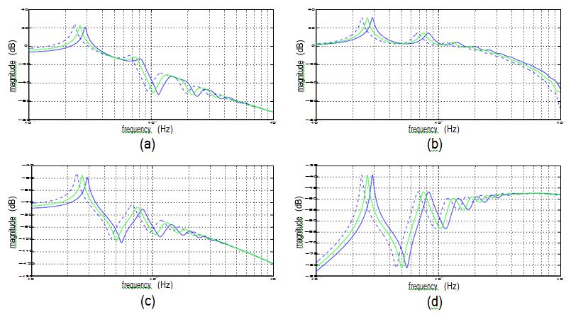
(a) ground excitation to roof horizontal displacement; (b) ground excitation to roof horizontal absolute acceleration; (c) horizontal force at roof to roof horizontal displacement; (d) horizontal force at roof to roof horizontal absolute acceleration (roof measurements taken at node-175).
Control Design Problem
The task of the designer/researcher in the benchmark study control design problem is to define an appropriate passive, active, or semi-active control strategy, or a combination thereof. It is left to the designer/researcher to define the type, appropriate model and location of the control device(s)/sensor(s) and to develop appropriate control algorithms. The evaluation model, how- ever, will remain invariant to the various applied control strategy. By using a single building model and common evaluation criteria, various control strategies can be compared directly to one another [14] [15].
Evaluation Criteria
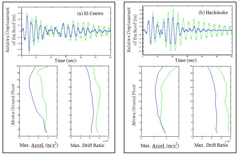
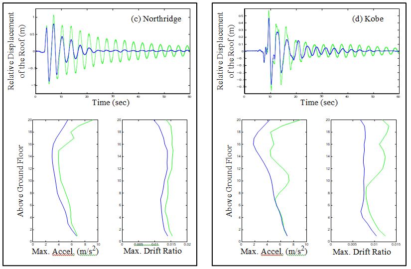
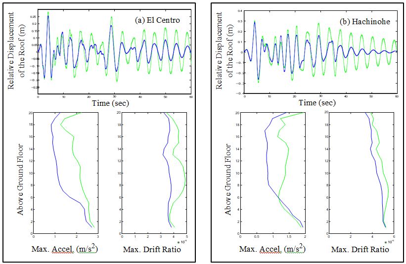
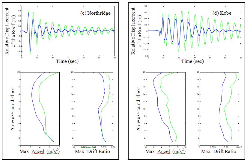
In evaluating proposed control strategies, the input excitation x˙˙g (m/sec2) is assumed to be one of the four historical earthquake records: (i) El Centro. The N-S component recorded at the Imperial Valley Irrigation District substation in El Centro, California, during the Imperial Valley, California earthquake of May, 18, 1940. (ii) Hachinohe. The N-S component recorded at Hachi- nohe City during the Takochi-oki earthquake of May, 16, 1968. (iii) Northridge. The N-S compo- nent recorded at Sylmar County Hospital parking lot in Sylmar, California, during the Northridge, California earthquake of January 17, 1994. (iv) Kobe. The N-S component recorded at the Kobe
You can download the Project files here: Download files now. (You must be logged in).
Japanese Meteorological Agency (JMA) station during the Hyogo-ken Nanbu earthquake of Janu- ary 17, 1995. Each proposed control strategy should be evaluated for all four earthquake records, with the appropriate responses being used to calculate the evaluation criteria for both the pre- earthquake and post-earthquake evaluation models. As detailed in the following paragraphs, the merit of a control strategy is based on criteria given in terms of maximum response quantities, as well as the number of sensors and control devices and the total power required by the control sys- tem. Smaller values of these evaluation criteria are generally more desirable.
Control Implementation Constraints and Procedures
To make the benchmark problem as representative of the full-scale implementation as possi- ble and to allow for direct comparison of the results submitted to the study, the following con- straints and procedures are specified:
- The measured outputs directly available for use in determination of the control action are the absolute horizontal acceleration and the interstory drift of each floor of the LA 20-story struc- ture, and control device outputs which are readily available (g., control device displacement,
Table 1: Uncontrolled Peak Response Quantities of the Pre- and Post-Earthquake Evaluation Models.
| El Centro | Hachinohe | Northridge | Kobe | |||||
| pre- earthquake | post- earthquake | pre- earthquake | post- earthquake | pre- earthquake | post- earthquake | pre- earthquake | post- earthquake | |
| xmax(m) | 0.37959 | 0.27787 | 0.51705 | 0.29831 | 1.0591 | 0.90765 | 0.56887 | 0.65617 |
| x˙max(m/sec) | 0.82539 | 0.74801 | 1.0450 | 0.76065 | 2.9023 | 2.6803 | 1.8370 | 1.6289 |
| x˙˙maxa (m/sec2) | 3.1372 | 2.8093 | 2.8439 | 1.9467 | 9.1886 | 7.7702 | 8.9544 | 7.7383 |
| dmax n | 6.2297×10⁻³ | 4.8655×10⁻³ | 7.6232×10⁻³ | 5.4667×10⁻³ | 15.644×10⁻³ | 18.484×10⁻³ | 13.353×10⁻³ | 14.223×10⁻³ |
| Fmaxb (kN) | 4.3525 x10⁶ | 2.0892 x10⁶ | 5.3852 x10⁶ | 2.6514 x10⁶ | 11.083 x10⁶ | 8.0311 x10⁶ | 9.4430 x10⁶ | 6.2433 x10⁶ |
| xmax(m × sec) | 0.80902 | 0.89099 | 1.4934 | 1.0881 | 2.4997 | 1.6861 | 0.99073 | 2.3438 |
| x˙˙maxa (m × sec–3 ¤ 2) | 4.7166 | 3.5697 | 5.7325 | 3.2852 | 10.329 | 8.8355 | 9.8980 | 9.5907 |
| dmax n( sec) | 1.2486 x10⁻² | 1.3707 x10⁻² | 2.2026 x10⁻² | 1.5781 x10⁻² | 3.7074 x10⁻² | 2.8271 x10⁻² | 1.7807 x10⁻² | 3.7656 x10⁻² |
| Fmaxb (kN × sec) | 8.8861 x10⁶ | 6.5488 x10⁶ | 15.5564 x10⁶ | 7.4806 x10⁶ | 26.247 x10⁶ | 13.464 x10⁶ | 12.913 x10⁶ | 17.986 x10⁶ |
force, or absolute acceleration). Although absolute velocity measurements are not available, they can be closely approximated by passing the measured accelerations through a second or- der filter as described in Spencer, et al. (1998).
- The digitally implemented controller has a sampling time of T = 005 sec.
- The A/D and D/A converters on the digital controller have 12-bit precision and a span of ±10
- Each of the measured responses contains an RMS noise of 03 Volts, which is approximately 0.3% of the full span of the A/D converters. The measurement noises are modeled as Gaussian rectangular pulse processes with a pulse width of 0.001 seconds.
- No hard limit is placed on the number of states of the control algorithm, although the number of states should be kept to a reasonable number as limited computational resources in the digi- tal controller exist. The designer/researcher should justify that the proposed algorithm(s) can be implemented with currently available computing hardware.
- The control algorithm is required to be
- The performance of each control design should be evaluated using both the 212 state pre-earth- quake evaluation model and the 212 state post-earthquake evaluation model for each of the earthquake records provided (e., El Centro, Hachinohe, Northridge and Kobe).
- The closed loop stability robustness for each proposed active control design should be dis-
- The control signal to each control device has a constraint of max ui(t ) £ 10 Volts for each re-spective earthquake. t
- The capabilities of each control device employed should be discussed, and the designer/re- searcher should provide a justification of the availability of each control device. Additional constraints unique to each control scheme should also be reported (g., maximum displace- ment, velocity, or force capacity of control devices).
- Designers/researchers should submit electronically a complete set of MATLAB files that will produce the evaluation criteria specified in this problem statement for both the pre- and post- earthquake evaluation For more details, see the README file included with the down- loaded benchmark data on the benchmark homepage (http://www.nd.edu/~quake/).
Sample Control System Design
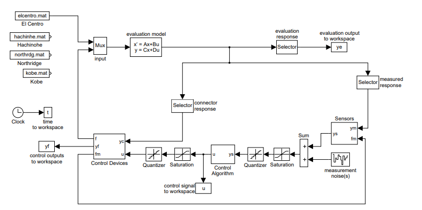
To illustrate some of the constraints and challenges of this benchmark problem, a sample control system is presented. The sample control system design is included to serve as a guide to the participants in this study and is not intended to be a competitive design. The sample control system is a type of active system that employs hydraulic actuators as control devices. Hydraulic actuators are located on each floor of the structure to provide control forces to the building. Feed- back measurements are provided by accelerometers placed at various locations on the structure. In this section, the accelerometers and hydraulic actuators chosen for the sample control system are described, and models for each are discussed. A linear quadratic Gaussian (LQG) control algo- rithm is designed based on a reduced order model of the system. The results are then discussed and the evaluation criteria are then determined for both the pre-earthquake and post-earthquake evaluation models.
Sensors
Because accelerometers can readily provide reliable and inexpensive measurements of the absolute accelerations of arbitrary points on a structure, the sample control system is based on acceleration feedback. A total of five acceleration measurements were selected for feedback in the control system (on floors 5, 9, 13, 17 and the roof).
You can download the Project files here: Download files now. (You must be logged in).
Conclusion
In conclusion, the Next Generation Benchmark Control Problem for Seismically Excited Buildings provides a standardized and comprehensive framework for evaluating the performance of different structural control strategies under realistic seismic loading conditions. By focusing on a 20-story steel building representative of typical mid- to high-rise structures in the Los Angeles region, the benchmark problem ensures that research outcomes are both practically relevant and scientifically rigorous. The inclusion of well-defined structural models, control constraints, and evaluation criteria enables fair and direct comparisons among passive, active, semi-active, and hybrid control systems. This approach addresses a longstanding gap in structural control research, where diverse methodologies have historically made cross-comparison challenging. The provision of a simulation program further facilitates collaborative research by allowing investigators to implement and test their designs in a controlled, repeatable environment. By encouraging participation from the global research community, the benchmark serves as a catalyst for innovation, helping to refine control algorithms, optimize sensor and actuator configurations, and improve the resilience of building structures to seismic hazards. Moreover, it fosters a deeper understanding of trade-offs between performance, cost, and complexity in structural control system design. As a result, the benchmark problem is expected to drive advancements not only in theoretical control strategy development but also in practical, deployable solutions for earthquake-prone regions. Ultimately, this coordinated effort enhances the potential for reducing structural damage, improving occupant safety, and extending the service life of critical infrastructure, aligning with the overarching goal of building safer and more resilient cities worldwide.
References
- Soong, T.T. (1990). Active Structural Control: Theory and Practice. Longman Scientific & Technical.
- Housner, G.W., et al. (1994). “Structural Control: Past, Present, and Future.” Journal of Engineering Mechanics, ASCE, 123(9), 897–971.
- Soong, T.T., and Constantinou, M.C. (1994). Passive and Active Structural Vibration Control in Civil Engineering. Springer.
- Fujino, Y., et al. (1996). “Passive and Active Structural Control in Japan.” Proceedings of the 2nd World Conference on Structural Control, Kyoto, Japan.
- Spencer, B.F., and Sain, M.K. (1997). “Controlling Buildings: A New Frontier in Feedback.” IEEE Control Systems Magazine, 17(6), 19–35.
- Dyke, S.J., et al. (1996). “Modeling and Control of Magnetorheological Dampers for Seismic Response Reduction.” Smart Materials and Structures, 5(5), 565–575.
- Christenson, R.E., et al. (2003). “Benchmark Control Problem for Seismically Excited Buildings.” Journal of Engineering Mechanics, 129(5), 509–516.
- Symans, M.D., et al. (2008). “Energy Dissipation Systems for Seismic Applications: Current Practice and Recent Developments.” Journal of Structural Engineering, 134(1), 3–21.
- Basu, B., et al. (2008). “Semi-active Control of Structures: A Review.” Journal of Structural Engineering, 134(1), 3–21.
- Spencer, B.F., Dyke, S.J., and Deoskar, H.S. (1998). “Benchmark Problems in Structural Control.” Journal of Structural Engineering, 124(4), 500–505.
- Nagarajaiah, S., and Narasimhan, S. (2006). “Seismic Control of Smart Structures Using Semi-active Control and Shape Memory Alloys.” Structural Control and Health Monitoring, 13(2–3), 573–593.
- Spencer, B.F., and Nagarajaiah, S. (2003). “State of the Art of Structural Control.” Journal of Structural Engineering, 129(7), 845–856.
- Dyke, S.J., et al. (1995). “Modeling and Control of MR Dampers for Seismic Response Reduction.” Proceedings of the American Control Conference, Seattle, WA.
- Johnson, E.A., et al. (1998). “Control Design Strategies for Buildings Subjected to Earthquakes.” Earthquake Engineering & Structural Dynamics, 27(10), 1121–1140.
- International Code Council (ICC). (2021). International Building Code. ICC, Washington, D.C.
You can download the Project files here: Download files now. (You must be logged in).


Responses