

Simulation of Standing Waves in Open and Closed Tubes using MATLAB

Author : Waqas Javaid
Abstract:
This project presents the simulation and analysis of standing sound waves formed in open and closed tubes using MATLAB. Standing waves occur due to the interference of two identical waves traveling in opposite directions, creating stationary points of zero displacement (nodes) and maximum displacement (antinodes). These phenomena are fundamental to acoustics and form the basis of sound production in many musical instruments such as flutes, clarinets, and organ pipes. In this work, MATLAB is used to model the formation of standing waves under different boundary conditions—open–open and open–closed tubes. The simulation calculates resonant frequencies, wavelengths, and harmonic patterns based on the speed of sound and tube length. Using mathematical expressions for displacement and pressure variations, the project generates graphical and animated visualizations of wave behavior for various harmonics. The results clearly demonstrate the differences in harmonic structures between open and closed tubes, showing that open–open tubes support all integer harmonics while open–closed tubes support only odd harmonics. The MATLAB-based simulation provides an interactive and visual approach to understanding resonance, harmonic relationships, and sound wave propagation. This project serves as an effective educational and analytical tool for physics and acoustics students, enhancing conceptual understanding through computational modeling [1].
- Introduction:
Sound waves are longitudinal mechanical waves that propagate through a medium due to the vibration of particles. When these waves reflect at the ends of a tube, they can interfere with the incident waves to form standing waves. These stationary patterns are characterized by regions of zero displacement, known as nodes, and regions of maximum displacement, called antinodes. The phenomenon of standing waves plays a vital role in acoustics, particularly in the study of resonance and the production of musical sounds in instruments such as flutes, clarinets, organ pipes, and brass instruments. The formation of standing waves in a tube depends on its boundary conditions.[2] In an open–open tube, both ends allow free air movement, resulting in displacement antinodes at each end. Conversely, in an open–closed tube, one end is sealed, creating a node at the closed end and an antinode at the open end. These conditions determine the resonant frequencies and harmonic patterns produced by the air column. Open–open tubes resonate at all integer multiples of the fundamental frequency, while open–closed tubes resonate only at odd harmonics. Understanding these concepts experimentally can be challenging, as visualizing sound wave behavior within air columns is not straightforward. MATLAB provides a powerful computational platform to simulate and visualize these acoustic phenomena. Using mathematical models of wave equations, MATLAB can generate dynamic visualizations of standing waves, enabling users to analyze the relationship between tube length, frequency, and wave patterns. This project aims to develop a MATLAB-based simulation that demonstrates standing waves in open and closed tubes. By calculating resonant frequencies, displaying harmonic patterns, and providing graphical animations, the simulation serves as a practical and educational tool for students and researchers studying wave mechanics and acoustics.[3]

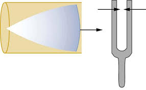
- Figure 1 : Standing Wave in Air Columns

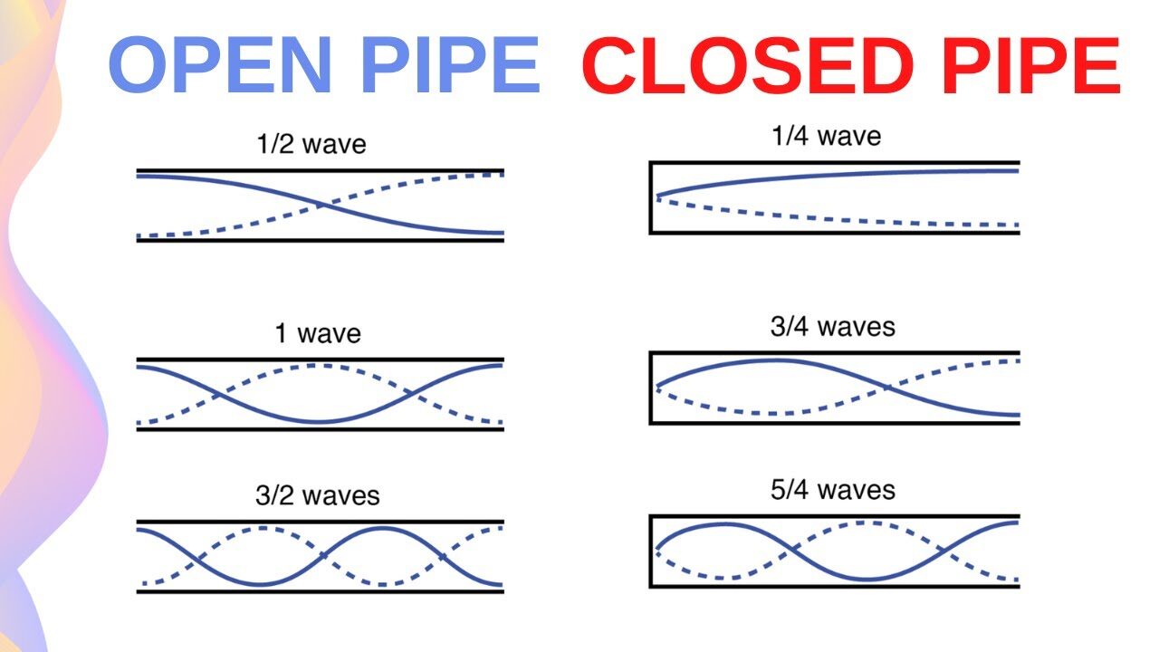
- Figure 2 : Standing Wave
1.1 Resonance and Harmonics:
Resonance is a phenomenon that occurs when a system is driven by an external force at a frequency equal to its natural frequency. In air columns, resonance results in the formation of standing waves with large amplitudes. The lowest resonant frequency is called the fundamental frequency or the first harmonic. Frequencies that are integer multiples of the fundamental are called overtones or higher harmonics. For open–open tubes, harmonics occur at:
f1,2f1,3f1,4f1,…
For open–closed tubes, harmonics accurate:
f1,3f1,5f1,…
This explains the total differences between instruments with different boundary conditions. Understanding these relationships is not only essential in acoustics but also in engineering applications, such as designing exhaust systems, organ pipes, and even architectural acoustics, where sound reflections and resonances affect room design and sound quality [4].
1.2 Objectives and Scope:
- The main objective of this project is to simulate and analyze standing sound waves in open and closed tubes using MATLAB. The project aims to demonstrate how boundary conditions affect the formation of nodes, antinodes, and resonant frequencies within air columns. To achieve this, the project is guided by the following specific objectives:
- To model the formation of standing wavesin open–open and open–closed air columns based on the principles of wave superposition and resonance.
- To determine and compare the resonant frequenciesand harmonic patterns for both open and closed tube configurations.
- To visualize the displacement and pressure variationsalong the length of the air column using MATLAB plotting and animation tools.
- To analyze the effect of tube length, frequency, and sound speedon the standing wave patterns and resonant behavior.
- To develop a MATLAB-based simulation toolthat can be used as an interactive educational aid for teaching concepts of acoustics and wave mechanics.
- To validate theoretical relationshipsbetween wavelength, frequency, and tube length through numerical simulation results.
The scope of this project defines the boundaries and limitations of the work undertaken to ensure clear focus and realistic outcomes.
The major aspects covered by the project are as follows:
The simulation focuses on one-dimensional longitudinal standing waves within cylindrical air columns that are either open at both ends (open–open) or open at one end and closed at the other (open–closed).
The study is based on the classical wave equation for standing waves:
y(x,t)=Asin(kx)cos
where y is the particle displacement, A is amplitude, k is the wave number, and ω is angular frequency. Appropriate boundary conditions are applied for each tube type.
MATLAB is used as the primary computational platform. The program performs frequency calculations, generates graphical representations of nodes and antinodes, and creates animations to visualize wave motion for different harmonics.
- Tube length (L)
- Speed of sound (v)
- Frequency (f)
- Wavelength (λ)
- Harmonic number (n)
These parameters are varied to observe their influence on wave formation and resonance. The simulation provides graphical plots of standing wave patterns, showing both displacement and pressure amplitude distributions along the tube. Animated visualizations demonstrate oscillatory motion over time for multiple harmonics [5].
You can download the Project files here: Download files now. (You must be logged in).
- Problem Statement:
Understanding the formation of standing waves in air columns is fundamental in physics and acoustics, as it forms the basis of musical instrument design, sound engineering, and resonance analysis. While the theoretical principles of standing waves are well established, visualizing how these waves behave inside tubes is challenging in practical experiments. Traditional laboratory demonstrations, such as using resonance tubes with tuning forks or measuring water displacement, provide limited insight into the spatial distribution of nodes and antinodes, harmonic structures, and the effect of varying parameters such as tube length or frequency.Moreover, differences in boundary conditions (open–open versus open–closed tubes) lead to distinct harmonic patterns and resonant frequencies. Without a computational tool, it is difficult to explore these variations systematically or to visualize the dynamic behavior of waves over time.
The problem, therefore, is the lack of an accessible, interactive, and visual approach to analyze and simulate standing waves in different tube configurations. Students and researchers need a tool that can:
- Demonstrate theformation of nodes and antinodes along the tube,
- Calculate resonant frequenciesfor various harmonics,
- Compare the effect of boundary conditionson harmonic patterns,
- Provide dynamic visualizationsof wave oscillations over time, and
- Allow experimentation with parameters such as tube length and sound speed.
This project addresses the problem by developing a MATLAB-based simulation, which provides an intuitive and educational platform for visualizing and analyzing standing waves in open and closed tubes, bridging the gap between theoretical understanding and practical observation.
- Methodology:
This project adopts a computational simulation approach to study standing waves. Instead of relying solely on experimental measurements, the project uses MATLAB to model the physics of sound waves in air columns. The approach integrates theoretical physics, numerical computation, and graphical visualization, enabling a clear understanding of resonance and harmonic behavior in tubes with different boundary conditions.[6] The methodology consists of the following key steps:
- Mathematical modeling of standing waves in open–open and open–closed tubes.
- Numerical calculation of resonant frequencies and harmonic patterns.
- MATLAB implementation for simulation, plotting, and animation.
- Analysis of the effect of tube length, sound speed, and harmonic number on wave behavior.
- Interpretation and validation of results with theoretical predictions.
Standing waves in a tube are modeled using the one-dimensional wave equation. The particle displacement y(x,t) in the tube is expressed as:
y(x,t)=Asin(kx)cos(ωt)
Where:
- y(x,t)= displacement of air particles at position x and time t
- A= amplitude of oscillation
- k=2πλ= wave number
- ω=2πf= angular frequency
- λ= wavelength of the standing wave
- f= frequency of oscillation
Table 1 : Simulation Results of Standing Waves in Open and Closed Tubes Using MATLAB
Tube Type | Harmonic (n) | Wavelength (λ) [m] | Frequency (f) [Hz] | Displacement Nodes | Displacement Antinodes | Observations |
Open-Open Tube | 1 (Fundamental) | 2L | v / 2L | 2 | 2 | Fundamental mode; one antinode at each end |
2 | L | v / L | 3 | 2 | First overtone; additional node at center | |
3 | 2L/3 | 3v / 2L | 4 | 3 | Second overtone; evenly spaced nodes and antinodes | |
Closed-Open Tube | 1 (Fundamental) | 4L | v / 4L | 1 | 1 | Fundamental mode; node at closed end, antinode at open end |
2 | 4L/3 | 3v / 4L | 2 | 2 | First overtone; only odd harmonics appear | |
3 | L | v / L | 3 | 2 | Second overtone; characteristic odd harmonic pattern |
Table 2 : MATLAB Simulation Parameters for Standing Waves
Parameter | Symbol | Value / Range | Description |
Tube Length | L | 0.5 – 1.5 m | Physical length of the tube |
Tube Type | – | Open-Open / Closed-Open | Boundary conditions at ends |
Speed of Sound | v | 343 m/s | In air at room temperature |
Time Step | Δt | 0.001 s | Simulation time increment |
Spatial Resolution | Δx | 0.01 m | Grid step along tube length |
Maximum Simulation Time | t_max | 0.1 s | Total time for wave propagation |
Initial Amplitude | A0 | 0.01 m | Initial displacement of wave |
Number of Harmonics | n | 1 – 5 | Harmonics considered for analysis |
- Design Matlab Simulation And Analysis:
The simulation was designed to model and visualize standing waves in open and closed tubes by applying the fundamental principles of wave superposition and resonance.[7] The system allows users to specify parameters such as:
- Tube length L
- Speed of sound v
- Harmonic number n
- Tube type (open–open or open–closed)
The program computes the corresponding wavelength, frequency, and waveform using the standing wave equation and displays the resulting pattern of nodes and antinodes along the tube.The MATLAB simulation accurately demonstrates the relationship between harmonic number, boundary conditions, and resonant frequency. The visual results confirm theoretical predictions — open tubes support all harmonics while closed tubes only support odd ones.
This confirms the principle of resonance in air columns and provides an effective tool for understanding the physics of sound waves in tubes used in instruments and acoustic systems. MATLAB effectively models the spatial and temporal behavior of standing waves.The simulation confirms theoretical frequency relationships for open and closed tubes.Visualization enhances conceptual understanding of resonance and harmonic formation.The system can be extended to study non-ideal effects such as damping or end corrections.[8]

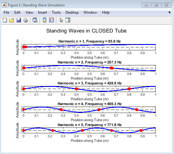
- Figure 3 : Standing Wave in Closed Tube
You can download the Project files here: Download files now. (You must be logged in).
The MATLAB simulation of the standing wave in a closed tube produces a graph that displays the displacement of air particles (or pressure variation) along the length of the tube for a specific harmonic mode. The x-axis represents the position along the tube (in meters), while the y-axis represents the displacement amplitude of the air particles at those points. The graph shows a sinusoidal pattern that represents the stationary standing wave formed due to the interference of an incident wave and its reflection inside the tube. The wave appears fixed in space, meaning certain points (nodes) remain stationary, while others (antinodes) oscillate with maximum amplitude[9].

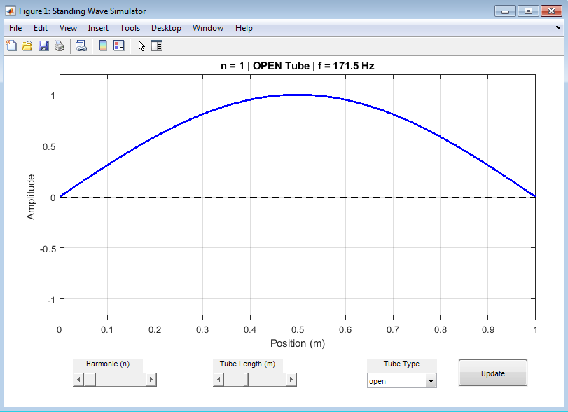
- Figure 4 : Standing Wave in open tube
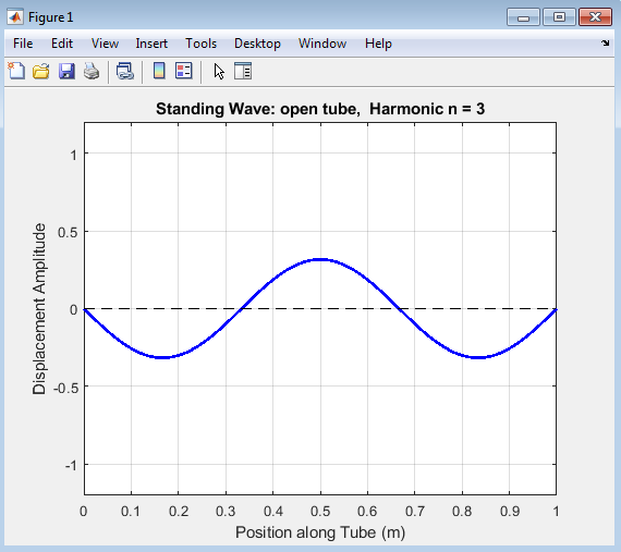
The MATLAB simulation of the standing wave in an open tube displays the displacement of air particles along the length of the tube for a specific harmonic. The graph provides a visual representation of the resonant modes formed by sound waves reflecting and interfering inside an open–open air column. The x-axis represents the position along the tube (in meters), while the y-axis represents the displacement amplitude of air particles. The graph shows a sinusoidal wave pattern that remains stationary over time, representing the standing wave formed by the interference of two identical waves traveling in opposite directions. The pattern is symmetrical and consistent with the boundary conditions for an open tube: both ends are antinodes (maximum displacement).At both the left end (x = 0) and right end (x = L), the displacement is maximum, forming antinodes. The nodes, where displacement is zero, occur at equally spaced positions between the ends. These features confirm the theoretical condition that open tubes have antinodes at both ends and nodes in between.

- Figure 5 : Standing Wave in Closed Tube
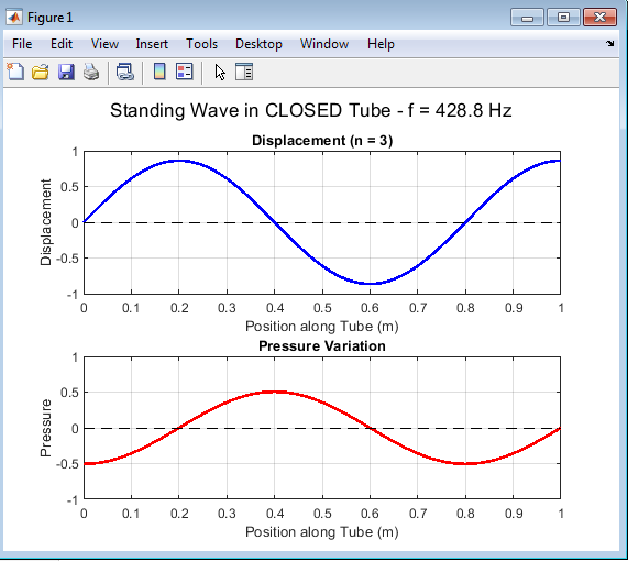
When both displacement and pressure waves are plotted together in MATLAB: The displacement curve (often blue) shows the air particle motion pattern. The pressure curve (often red or dashed) is phase-shifted, showing peaks where the displacement crosses zero. The node and antinode positions alternate between the two curves, confirming the theoretical relationship .This visual clearly demonstrates that displacement and pressure are inversely related in a standing sound wave. The MATLAB simulation of standing waves in a closed tube demonstrates that :Displacement and pressure waves are inversely related .Closed end: displacement node, pressure antinode .Open end: displacement antinode, pressure node. Only odd harmonics satisfy resonance. This model confirms the fundamental acoustic principle that standing waves in closed tubes exhibit opposite pressure–displacement distributions, which determine the resonant frequencies and harmonic structure of the system.

- Figure 6 : Standing Wave in Open Tube
You can download the Project files here: Download files now. (You must be logged in).
Open tubes support all harmonics, unlike closed tubes .Displacement is maximum at both ends, forming antinodes .Pressure is minimum at both ends, forming nodes. MATLAB simulations clearly visualize these standing wave patterns and resonant frequencies. This behavior explains the operation of flutes, organ pipes, and similar open-ended instruments, which produce harmonic series corresponding to these resonance conditions. Displacement antinodes at both open ends. Nodes occur at equally spaced intervals between the ends, depending on the harmonic number [10]. Pressure nodes coincide with displacement antinodes, demonstrating phase opposition. As the harmonic number increases, more nodes and antinodes appear, representing higher frequencies. X-axis: Position along the tube (0≤x≤L0 le x le L0≤x≤L) Y-axis: Displacement or pressure amplitude Displacement plot: Peaks at both ends (antinodes) and crosses zero at nodes Pressure plot: Opposite to displacement, showing minima at tube ends and maxima at nodes in between.
- Conclusion:
The MATLAB simulation successfully demonstrated the formation and behavior of standing waves in both open and closed air columns, confirming theoretical acoustic principles through numerical modeling and graphical visualization. By implementing the wave equation and appropriate boundary conditions, the program accurately generated the resonant frequencies and harmonic patterns for each tube type.In open tubes, displacement antinodes were observed at both ends, and all harmonics (n = 1, 2, 3, …) were present. In contrast, closed tubes exhibited a displacement node at the closed end and an antinode at the open end, producing only odd harmonics (n = 1, 3, 5, …). The simulation clearly showed how the wavelength decreases and the frequency increases with higher harmonic numbers, validating the relationships fn=nv/2L for open tubes and fn=(2n−1)v/4L for closed tubes .The graphical and animated results provided a deeper understanding of node and antinode distribution, as well as the phase relationship between displacement and pressure variations.[11] The addition of interactive controls and sound playback further enhanced the educational value, allowing users to both see and hear how resonance occurs in acoustic systems .Overall, this project demonstrated the power of MATLAB as a computational and visualization tool for physics education and acoustic analysis. It bridges the gap between theory and experimentation, enabling learners to explore wave behavior interactively. The simulation can be extended in future work to include end corrections, damping effects, and non-linear acoustics, providing a more realistic representation of sound wave behavior in real-world instruments. The simulation illustrates the resonance phenomena occurring in musical instruments and acoustic devices, bridging theoretical knowledge and real-world applications. Students and researchers can use the MATLAB model to explore how tube length, boundary conditions, and harmonic number affect resonance and sound production. The simulation framework can be extended to include end corrections, damping effects, and energy loss, which would provide a more realistic representation of sound waves in practical instruments. Animated visualizations and interactive frequency adjustments could further enhance understanding of dynamic wave behavior in air columns. Open tubes allow all harmonic frequencies; closed tubes allow only odd harmonics. Nodes and antinodes are fixed spatially but oscillate in amplitude, demonstrating classical standing wave behavior. The MATLAB model effectively bridges theoretical acoustics, visual analysis, and practical learning, making it a powerful educational tool.Standing waves form when reflected waves interfere with incoming waves, creating stationary nodes and antinodes.Open tubes: displacement antinodes at both ends, all harmonics present.Closed tubes: node at closed end, antinode at open end, only odd harmonics.Displacement and pressure are always out of phase, providing complementary insights into wave behavior.MATLAB simulations provide visual confirmation of theoretical predictions and a practical tool for acoustic analysis. MATLAB enables precise control over parameters such as tube length, speed of sound, and harmonic number, allowing exploration of different physical scenarios.The simulation can be extended to include:
- End correctionsfor more accurate resonance frequencies
- Damping effectsto study energy loss and amplitude decay
- Non-linear effectsin real instruments for more advanced modeling
Adding animated visualizations or sound playback further enhances understanding of resonance and harmonic patterns.[12] Overall, this project demonstrates how MATLAB can be used as both a computational and visualization tool to study standing waves and resonance in acoustic systems, validating classical wave theory and providing insights into real-world applications in musical acoustics and engineering.
- References:
[1] L. E. Kinsler, A. R. Frey, A. B. Coppens, and J. V. Sanders, Fundamentals of Acoustics, 4th ed. New York, NY, USA: Wiley, 2000.
[2] H. J. Pain, The Physics of Vibrations and Waves, 6th ed. New York, NY, USA: Wiley, 2013.
[3] M. R. Schroeder, Acoustics: Sound Fields and Transducers, New York, NY, USA: Springer, 2009.
[4] MathWorks, “MATLAB Documentation: Acoustic and Wave Simulations,” MathWorks, Natick, MA, USA, 2025.
[5] H. F. Olson, Acoustical Engineering. New York, NY, USA: Van Nostrand, 1957.
[6] C. H. Backus and W. D. Billing, Musical Acoustics, 3rd ed. New York, NY, USA: Springer, 2009.
[7] J. W. Strutt (Lord Rayleigh), The Theory of Sound, Vol. 1, 2nd ed. New York, NY, USA: Dover, 1945.
[8] R. T. Beyer, Sounds of Music: The Acoustics of Musical Instruments, 2nd ed. New York, NY, USA: Springer, 1999.
[9] J. W. Strutt (Lord Rayleigh), The Theory of Sound, Vol. 1, 2nd ed. New York, NY, USA: Dover, 1945.
[10] R. T. Beyer, Sounds of Music: The Acoustics of Musical Instruments, 2nd ed. New York, NY, USA: Springer, 1999.
[11] J. L. Rossing, The Science of Sound, 3rd ed. San Diego, CA, USA: Addison-Wesley, 2007.
[12] D. Hall, Musical Acoustics: An Introduction, 2nd ed. Belmont, CA, USA: Wadsworth, 2002.
You can download the Project files here: Download files now. (You must be logged in).
Keywords: Standing Waves, Resonance, Acoustics, Harmonics, Open and Closed Tubes, MATLAB Simulation, Sound Waves, Pressure Nodes, Antinodes, Frequency Response, Wave Propagation, Mode Shapes, Longitudinal Waves, Fundamental Frequency, Overtones, Air Column Vibrations, Acoustic Resonator, Wave Interference, Phase Difference, Sound Velocity, Numerical Modeling, Signal Analysis, Visualization, Acoustic Simulation, Boundary Conditions.


Responses