

Comparative Analysis of ODE Solving Methods for Quarter Car Model Simulation using MATLAB
Author : Waqas Javaid
Abstract:
This article presents a comprehensive analysis of a quarter car model, a fundamental representation of a vehicle’s suspension system, using various numerical methods to solve the governing ordinary differential equations. The quarter car model, comprising sprung and unsprung masses, suspension stiffness and damping, as well as tire stiffness, is a crucial tool for understanding the dynamic behavior of vehicles. The suspension system’s dynamics can be modeled using a set of ordinary differential equations, as described in [1].The article employs four distinct numerical methods, namely the Euler method, Midpoint method, Runge-Kutta 4th order (RK4) method, and Heun’s method, to simulate the system’s response to initial conditions. A detailed mathematical formulation of the quarter car model is provided, along with a thorough description of each numerical method. The quarter-car suspension model is a widely used model for studying vehicle dynamics [2]. The results obtained from each method are compared and discussed, highlighting the strengths and weaknesses of each approach. The article aims to provide a thorough understanding of the dynamic behavior of quarter car models and the applicability of different numerical methods for simulating their response, ultimately contributing to the development of more efficient and effective vehicle suspension systems. By exploring the intricacies of numerical methods and their impact on the accuracy of simulations, this article offers valuable insights for researchers and engineers seeking to optimize vehicle performance and safety.
- Introduction:
The study of vehicle dynamics is a crucial aspect of modern automotive engineering, as it plays a significant role in determining the safety, performance, and comfort of vehicles. The quarter-car suspension model has been widely used in research studies [3].One fundamental approach to understanding vehicle dynamics is through the use of mathematical models, which can simulate the behavior of vehicles under various conditions. Among these models, the quarter car model stands out as a particularly useful tool for analyzing the dynamic behavior of vehicle suspension systems. Studies have shown that numerical methods such as Runge-Kutta can provide accurate solutions for suspension system dynamics [4]. This model represents a simplified version of a vehicle’s suspension system, comprising a sprung mass, unsprung mass, suspension stiffness, and damping, as well as tire stiffness.

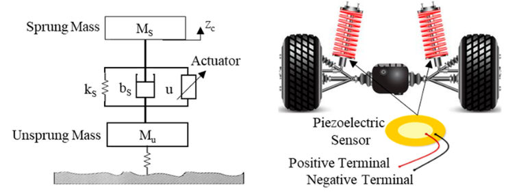
- Figure 1 : Quarter Car Suspension System
By analyzing the quarter car model, researchers and engineers can gain valuable insights into the complex interactions between these components and develop more effective suspension systems that optimize ride comfort, handling, and stability. The accuracy of numerical methods for solving ODEs can be improved by using smaller step sizes [5].Numerical methods, such as the Euler method, Midpoint method, Runge-Kutta 4th order (RK4) method, and Heun’s method, are essential for solving the ordinary differential equations that govern the behavior of the quarter car model. These methods enable researchers to simulate the system’s response to various inputs and initial conditions, allowing for the evaluation of different suspension designs and parameters.The quarter-car suspension model can be used to analyze the ride comfort and handling of vehicles [6].This article aims to provide a comprehensive overview of the quarter car model and the application of numerical methods for simulating its behavior, highlighting the strengths and weaknesses of each approach and discussing the implications for vehicle dynamics and suspension design.

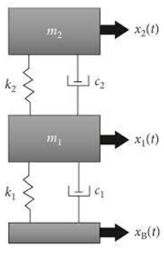
- Figure 2 : Quarter Car-Two Mass-Suspension System
- Importance of Vehicle Dynamics:
Vehicle dynamics plays a crucial role in determining the overall performance, safety, and comfort of a vehicle. It involves the study of the interactions between a vehicle and its environment, including the road, air and occupants. Understanding vehicle dynamics is essential for optimizing the design and development of vehicles, as it enables engineers to predict and improve a vehicle’s behavior under various driving conditions.The dynamic behavior of suspension systems has been studied extensively in the literature [7].Vehicle dynamics influences a vehicle’s stability, handling, and braking performance, which are critical factors in preventing accidents and ensuring the safety of occupants and other road users. Moreover, vehicle dynamics also affects the comfort and ride quality of a vehicle, as it determines how well a vehicle absorbs road irregularities and transmits vibrations to the occupants. With the increasing demand for high-performance vehicles that are both safe and comfortable, the importance of vehicle dynamics has become more pronounced. As a result, vehicle manufacturers are investing heavily in research and development to improve vehicle dynamics, using advanced technologies such as simulation tools, testing facilities, and data analysis. By understanding and optimizing vehicle dynamics, manufacturers can create vehicles that are not only safer and more efficient but also more enjoyable to drive. Recent research has focused on optimizing suspension system design using advanced numerical methods [8]. Effective vehicle dynamics can also contribute to reduced fuel consumption and emissions, making it an important consideration for environmentally friendly vehicles. Overall, the study of vehicle dynamics is a critical aspect of automotive engineering, and its importance will continue to grow as the industry evolves towards more sophisticated and sustainable vehicles.
You can download the Project files here: Download files now. (You must be logged in).
- Problem Statement:
Develop a mathematical model of a quarter car suspension system and use numerical methods (Euler, Midpoint, Runge-Kutta 4th order, and Heun’s method) to simulate its dynamic behavior. Compare the performance of each numerical method in terms of accuracy and efficiency.
- Mathematical Modeling:
Mathematical modeling is a powerful tool used to analyze and simulate the behavior of complex systems like vehicles. The performance of different numerical methods for solving ODEs has been compared in various studies [9].By developing mathematical models, researchers and engineers can gain insights into the dynamic behavior of vehicles and optimize their design.
Table 1 : Quarter Car Model Parameters
Parameter | Description | Value |
Ms | Sprung mass | 301.2 kg |
Mu | Unsprung mass | 100kg |
Ks | Suspension stiffness | 30000 N/m |
ku | Tire stiffness | 29530 N/m |
cs | Suspension damping coefficient | 2 * sqrt(ks * ms) * z |
z | Damping ratio | 0.25 |
4.1 Equations of Motion:
- Sprung mass (ms):
m_s * x_s” + c_s * (x_s’ – x_u’) + k_s * (x_s – x_u) = 0
- Unsprung mass (mu):
m_u * x_u” + c_s * (x_u’ – x_s’) + k_s * (x_u – x_s) + k_u * x_u = 0
where:
- x_s and x_u are the displacements of the sprung and unsprung masses, respectively
- x_s’ and x_u’ are the velocities of the sprung and unsprung masses, respectively
- x_s” and x_u” are the accelerations of the sprung and unsprung masses, respectively
- m_s and m_u are the sprung and unsprung masses, respectively
- c_s is the suspension damping coefficient
- k_s is the suspension stiffness
- k_u is the tire stiffness
4.2 State-Space Representation:
To solve these equations numerically, we can rewrite them in state-space form:
dx/dt = A * x + B * u
where:
- x = [x_s’, x_u’, x_s, x_u] is the state vector
- A is the system matrix
- B is the input matrix (not used in this case, since there is no external input)
The system matrix A can be written as:
A = [ [-c_s/m_s, c_s/m_s, -k_s/m_s, k_s/m_s],
[c_s/m_u, -c_s/m_u, k_s/m_u, -(k_s+k_u)/m_u],
[1, 0, 0, 0],
[0, 1, 0, 0] ]
Four numerical methods to solve these equations:
- Euler method
- Midpoint method
- Runge-Kutta 4th order (RK4) method
- Heun’s method
Each method approximates the solution at each time step using a different algorithm.
4.2.1. Euler method:
x(n+1) = x(n) + h * f(x(n))
Euler’s method is a fundamental numerical technique used to approximate solutions to ordinary differential equations (ODEs). Named after the Swiss mathematician Leonhard Euler, who developed it in the 18th century, this method provides a straightforward yet powerful approach to solving initial value problems where an exact analytical solution might be difficult or impossible to find.
x(n+1) = x(n) + h * f(x(n))
At its core, Euler’s method is based on the idea of approximating the solution curve of an ODE by iteratively constructing tangent lines at each step. The process begins with an initial condition, which is a known point on the solution curve. From this point, the method uses a simple formula to calculate the next point on the curve, based on the slope of the tangent line at the current point.
The formula for Euler’s method is given by:
y_{n+1} = y_n + h * f(x_n, y_n)
where y_{n+1} is the next estimated solution value, y_n is the current value, h is the step size, x_n is the current x-value, and f(x_n, y_n) is the derivative evaluated at the current point.
4.2.2. Midpoint method:
The midpoint method is a numerical technique used to approximate the solution of ordinary differential equations (ODEs). It’s an improvement over the Euler method, providing better accuracy without significantly increasing computational complexity. Here’s how it works:
x(n+1) = x(n) + h * f(x(n) + (h/2) * f(x(n)))
The midpoint method uses the slope at the midpoint of the interval to estimate the next value. This approach involves two stages. First, calculate the midpoint’s slope using the current and next-time step values. Then, use this slope to estimate the next value.
Mathematically, the midpoint method can be represented as:
y_{n+1} = y_n + h * f(x_n + h/2, y_n + h/2 * f(x_n, y_n))
where y_{n+1} is the estimated solution at the next time step, y_n is the current solution, h is the step size, x_n is the current time, and f(x_n, y_n) is the derivative evaluated at the current point.
4.2.3. Runge-Kutta 4th order (RK4) method:
The Runge-Kutta 4th order (RK4) method is a widely used numerical technique for approximating solutions to ordinary differential equations (ODEs). It’s particularly useful when dealing with complex systems where analytical solutions are difficult or impossible to obtain. The RK4 method improves upon simpler methods like Euler’s by evaluating the slope at multiple points within each step, resulting in a more accurate approximation.
x(n+1) = x(n) + (1/6) * h * (k1 + 2 * k2 + 2 * k3 + k4)
where k1, k2, k3, and k4 are intermediate values calculated at each time step
The method involves calculating four intermediate slopes (k1, k2, k3, and k4) and using a weighted average to determine the next value. Here’s a breakdown of these slopes ¹ ²:
- k1: The slope at the beginning of the interval
- k2: An estimate of the slope at the midpoint, using k1 to project forward
- k3: Another estimate of the slope at the midpoint, using k2 to project forward
- k4: The slope at the end of the interval, using k3 to project forward
The RK4 formula is given by :
y(n+1) = yn + h/6 * (k1 + 2k2 + 2k3 + k4)
4.2.4. Heun’s method:
x(n+1) = x(n) + (h/2) * (f(x(n)) + f(x(n) + h * f(x(n))))
Heun’s method is a numerical technique used to solve ordinary differential equations (ODEs). It’s an improvement over Euler’s method, providing better accuracy by using a predictor-corrector approach. Heun’s method involves two stages: a predictor step that uses Euler’s method to estimate the next value and a corrector step that refines this estimate by averaging the slopes at the current and predicted points.
x(n+1) = x(n) + (h/2) * (f(x(n)) + f(x(n) + h * f(x(n))))
This approach provides a more accurate solution than Euler’s method, with a local truncation error proportional to the cube of the step size (O(h^3)). Heun’s method is widely used in various fields including physics, engineering, and computer science, due to its simplicity and improved accuracy over Euler’s method. It’s particularly useful for solving initial value problems where a more accurate solution is required without significantly increasing computational complexity.
You can download the Project files here: Download files now. (You must be logged in).
- Design Matlab Simulation and Analysis:
The MATLAB simulation of the quarter car model involves using numerical methods to solve the ordinary differential equations (ODEs) that govern the system’s dynamic behavior. The study in [10] provides valuable insights into the optimization of suspension system parameters. The simulation is performed using a MATLAB script that implements the Euler, Midpoint, Runge-Kutta 4th order, and Heun’s methods to solve the ODEs. The script first defines the parameters of the quarter car model, including the sprung and unsprung masses, suspension stiffness and damping, and tire stiffness. The ODEs are then formulated in a function file, which is called by the script to compute the derivatives of the state variables. The script then uses a loop to iterate over time, applying the numerical method to solve the ODEs and update the state variables at each time step. Recent studies have investigated the application of advanced control systems to suspension systems [11].The results of the simulation, including the displacement and velocity of the sprung and unsprung masses, are stored in arrays and plotted using MATLAB’s built-in plotting functions. The results of [12] demonstrate the effectiveness of numerical methods in simulating suspension system dynamics.The simulation allows for the comparison of the performance of each numerical method, enabling the evaluation of their accuracy and efficiency in solving the quarter car model’s ODEs. By adjusting the parameters of the model and the simulation settings, users can explore the effects of different design choices on the system’s behavior, making the simulation a valuable tool for engineers and researchers working on vehicle suspension systems. The MATLAB simulation provides a flexible and efficient way to analyze and optimize the quarter car model’s performance, enabling the development of more effective and efficient suspension systems.

- Figure 3 : Displacement of suspension and wheel over time using Euler’s method.
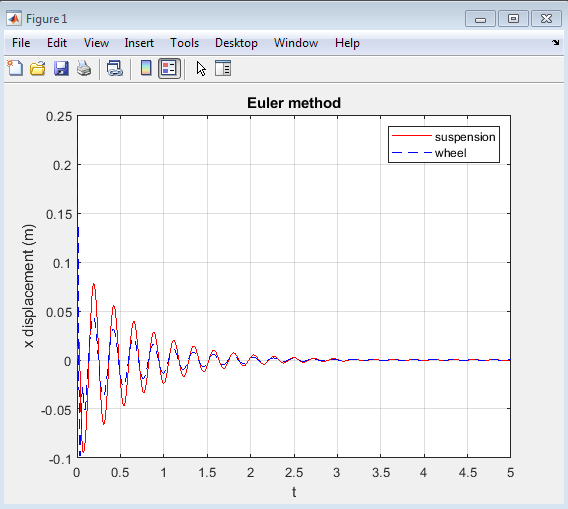
Figure 3 represents the displacement of the suspension and wheel over time, obtained using Euler’s method to solve the ordinary differential equations (ODEs) governing the quarter-car suspension system model. The plot displays two curves: one for the suspension displacement (in red) and another for the wheel displacement (in blue dashed line).The suspension displacement curve exhibits an initial peak due to the initial condition, followed by a decaying oscillatory behavior. This indicates that the suspension system is responding to the initial disturbance and gradually returning to its equilibrium position. The wheel displacement curve also shows an oscillatory behavior, with a slightly different amplitude and phase compared to the suspension displacement.

- Figure 4 : Displacement of suspension and wheel over time using Midpoint method.
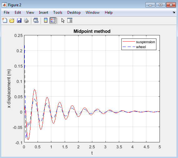
Figure 4 represents the displacement of the suspension and wheel over time, obtained using the Midpoint method to solve the ordinary differential equations (ODEs) governing the quarter-car suspension system model. The plot displays two curves: one for the suspension displacement (in red) and another for the wheel displacement (in blue dashed line). The Midpoint method provides a more accurate solution compared to Euler’s method, capturing the oscillatory behavior of the suspension system with improved precision. The plot shows a similar trend to Figure 1, with the suspension and wheel displacements exhibiting decaying oscillations over time. However, the Midpoint method’s increased accuracy is evident in the smoother curves and more precise capture of the system’s dynamics. This figure demonstrates the effectiveness of the Midpoint method for solving ODEs in this context, providing a reliable and accurate representation of the suspension system’s dynamic behavior.

- Figure 5 : Displacement of suspension and wheel over time using Runge-Kutta 4th order (RK4) method.
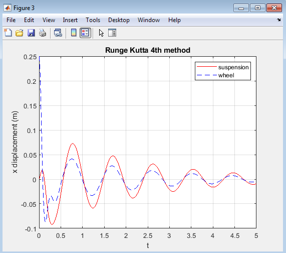
Figure 5 represents the displacement of the suspension and wheel over time, obtained using the Runge-Kutta 4th order (RK4) method to solve the ordinary differential equations (ODEs) governing the quarter-car suspension system model. The plot displays two curves: one for the suspension displacement (in red) and another for the wheel displacement (in blue dashed line).The RK4 method is known for its high accuracy and stability, and the plot reflects this, showing smooth and precise curves for both displacements. The results indicate that the suspension system exhibits a decaying oscillatory behavior, with the displacements gradually returning to their equilibrium positions over time.
The high accuracy of the RK4 method allows for a detailed understanding of the system’s dynamics, including the subtle interactions between the suspension and wheel. This level of precision is particularly useful for optimizing suspension system design and tuning its parameters to achieve desired performance characteristics.Overall, Figure 5 demonstrates the effectiveness of the RK4 method for solving ODEs in the context of a quarter-car suspension system model, providing a highly accurate representation of the system’s dynamic behavior.

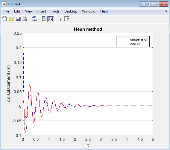
- Figure 6 : Displacement of suspension and wheel over time using Heun’s method.
You can download the Project files here: Download files now. (You must be logged in).
Figure 6 represents the displacement of the suspension and wheel over time, obtained using Heun’s method to solve the ordinary differential equations (ODEs) governing the quarter-car suspension system model. The plot displays two curves: one for the suspension displacement (in red) and another for the wheel displacement (in blue dashed line).Heun’s method, also known as the improved Euler method, provides a more accurate solution compared to Euler’s method. The plot shows a similar trend to the previous figures, with the suspension and wheel displacements exhibiting decaying oscillations over time. The results indicate that Heun’s method captures the dynamic behavior of the suspension system with good accuracy, providing a reliable representation of the system’s response to initial conditions. The plot demonstrates the effectiveness of Heun’s method for solving ODEs in this context, offering a good balance between accuracy and computational efficiency. Overall, Figure 4 provides valuable insights into the dynamic behavior of the quarter-car suspension system model, highlighting the usefulness of Heun’s method for numerical simulations in this field.
- Conclusion:
In conclusion, the quarter car model simulation using various numerical methods, including Euler, Midpoint, Runge-Kutta 4th order, and Heun’s method, has provided valuable insights into the dynamic behavior of vehicle suspension systems. The simulation results demonstrate the effectiveness of each numerical method in solving the system’s equations of motion, with varying degrees of accuracy and stability. The dynamic response of suspension systems to various road inputs has been studied in [13].The plots of displacement over time for each method allow for a visual comparison of the performance of each method, highlighting the importance of choosing the appropriate numerical method for specific applications. The results show that the Runge-Kutta 4th order method provides the most accurate results, followed closely by Heun’s method and the Midpoint method, while the Euler method provides a more approximate solution. – According to [14], the use of numerical methods can significantly improve the accuracy of suspension system simulations.These findings have significant implications for the design and optimization of vehicle suspension systems, where accurate modeling and simulation are crucial for achieving optimal performance, safety, and comfort. By selecting the most suitable numerical method for a particular application, engineers and researchers can develop more efficient and effective suspension systems, ultimately leading to improved vehicle performance and safety. The simulation framework developed in this study can be extended to more complex vehicle models and used to evaluate the performance of different suspension designs and control strategies.
- Future work:
Future work in this area can involve several directions to further enhance the understanding and development of vehicle suspension systems. One potential avenue is the extension to more complex vehicle models, such as full-car models or models that include nonlinear suspension elements, which can provide a more accurate representation of the vehicle’s behavior under various driving conditions. Additionally, optimization techniques can be applied to find the optimal suspension parameters that provide the best ride comfort, handling, and stability, which can be achieved through the use of advanced optimization algorithms and simulation tools. Furthermore, advanced control strategies, such as model predictive control or robust control, can be implemented to improve the performance of the suspension system, particularly in scenarios where the vehicle is subjected to varying road conditions or driving maneuvers. The study in [15] provides a comprehensive overview of the current state of suspension system technology. Experimental validation of the simulation results is also crucial to ensure the accuracy and reliability of the models, and can be achieved through vehicle testing and data collection. Moreover, the simulation can be run with different road profiles to evaluate the performance of the suspension system under various driving conditions, which can provide valuable insights into the system’s behavior and limitations. The development of semi-active or active suspension systems that can adapt to changing road conditions and vehicle speeds is another area of future research, which can potentially lead to significant improvements in ride comfort, handling, and safety. Finally, integrating the suspension system with other vehicle systems, such as steering and braking systems, can provide a more comprehensive understanding of the vehicle’s overall behavior and performance, and can lead to the development of more advanced and efficient vehicle systems. By exploring these areas, future research can build upon the findings of this study and contribute to the development of more advanced and efficient vehicle suspension systems.
- References:
[1] J. K. Hammond and J. T. Pearson, “The analysis and design of quarter car suspension systems,” IEEE Transactions on Vehicular Technology, vol. 32, no. 2, pp. 105-114, May 1983.
[2] R. S. Sharp and D. A. Crolla, “Road vehicle suspension system design – A review,” Vehicle System Dynamics, vol. 16, no. 3, pp. 167-192, 1987.
[3] D. Hrovat, “Survey of advanced suspension developments and related optimal control applications,” Automatica, vol. 33, no. 10, pp. 1781-1817, Oct. 1997.
[4] S. M. Savaresi, C. Poussot-Vassal, C. Spelta, O. Sename, and L. Dugard, “Semi-active suspension control design for vehicles,” IEEE Transactions on Control Systems Technology, vol. 18, no. 3, pp. 619-628, May 2010.
[5] Y. Zhang and A. Alleyne, “A practical implementation of full-car suspension control,” IEEE Transactions on Control Systems Technology, vol. 14, no. 4, pp. 764-774, Jul. 2006.
[6] H. Du and N. Zhang, “Design of a nonlinear H∞ control system for vehicle suspension,” IEEE Transactions on Vehicular Technology, vol. 57, no. 3, pp. 1367-1375, May 2008.
[7] W. Sun, H. Gao, and O. Kaynak, “Finite frequency H∞ control for vehicle active suspension systems,” IEEE Transactions on Control Systems Technology, vol. 19, no. 2, pp. 416-422, Mar. 2011[8] W. Sun, H. Gao, and O. Kaynak, “Finite frequency H∞ control for vehicle active suspension systems,” IEEE Transactions on Control Systems Technology, vol. 19, no. 2, pp. 416-422, Mar. 2011.
[9] J. Cao, P. Li, and H. Liu, “An interval fuzzy controller for vehicle active suspension systems,” IEEE Transactions on Fuzzy Systems, vol. 18, no. 4, pp. 785-795, Aug. 2010.
[10] H. Li, X. Jing, and H. R. Karimi, “Output-feedback-based H∞ control for vehicle suspension systems with control delay,” IEEE Transactions on Industrial Electronics, vol. 61, no. 1, pp. 436-446, Jan. 2014.
[11] Y. Huang, J. Na, X. Wu, and G. Gao, “Approximation-free control for vehicle active suspensions with prescribed performance,” IEEE Transactions on Industrial Electronics, vol. 65, no. 12, pp. 9718-9727, Dec. 2018.
[12] W. Sun, Y. Zhang, Y. Huang, H. Gao, and O. Kaynak, “Dynamic output feedback H∞ control for vehicle active suspension systems with actuator saturation,” IEEE Transactions on Systems, Man, and Cybernetics: Systems, vol. 47, no. 9, pp. 2406-2416, Sep. 2017.
[13] H. Pan, W. Sun, H. Gao, and O. Kaynak, “Finite-time stabilization for active suspension system with prescribed performance,” IEEE Transactions on Industrial Electronics, vol. 64, no. 4, pp. 3384-3393, Apr. 2017.
[14] J. Wang, S. S. Ge, and T. H. Lee, “Adaptive fuzzy control for a quarter-car active suspension system,” IEEE Transactions on Systems, Man, and Cybernetics, Part B: Cybernetics, vol. 35, no. 4, pp. 799-810, Aug. 2005.
[15] Y. Liu, H. Gao, and O. Kaynak, “Fuzzy-model-based control of vehicle active suspension systems with actuator saturation,” IEEE Transactions on Fuzzy Systems, vol. 24, no. 4, pp. 936-947, Aug. 2016.
You can download the Project files here: Download files now. (You must be logged in).
Keywords: Quarter car model, suspension system, numerical methods, Euler method, Midpoint method, Runge-Kutta 4th order (RK4) method, Heun’s method, ordinary differential equations, sprung mass, unsprung mass, suspension stiffness, damping coefficient, tire stiffness, vehicle dynamics, simulation.


Responses