

Optimal Siting and Sizing of Distributed Generation in Radial Distribution System using Genetic Algorithm

Author: Waqas Javaid
ABSTRACT
The demand for electrical power is growing at a rapid pace and the gap between generation and load is increasing. The difference between demand and load leads to several problems like outages, poor power quality and even sometimes to black out. These problems can be solved by the introduction of Distributed Generation (DG) in the system. For maximum reliability, technical and economical advantages, proper sizing or capacity of distributed generators, its proper allocation in the power systems, types of generating unit, number of units etc. are very important. Among these factors, the problem of installation of DG units with optimal location and size is of great importance. Improper allocation of DG resources in power system would lead to increase in power losses .Genetic algorithm is used as a solving tool for tackling this optimization problem. Load flow for standard 15 bus radial distribution system is developed using the Backward Forward sweep method. The impact of DG size and location on system losses is studied using load flow. Improper allocation of DG leads to increase in system losses. Hence, Genetic algorithm (GA), an evolutionary method, is studied and an algorithm is developed to find the optimal size and location of distributed generation unit in a radial distribution system. The total active power losses are minimized and voltage profile is improved by the proper allocation of DG. Multi objective function is introduced which includes the active power losses, the voltage deviation and DG cost with appropriate weight of each variable. Minimization of objective function is subjected to voltage constraints, active power losses constraints and DG size constraints. This method is implemented on the standard 15 bus radial distribution system.
1. INTRODUCTION
1.1 Indian power scenario
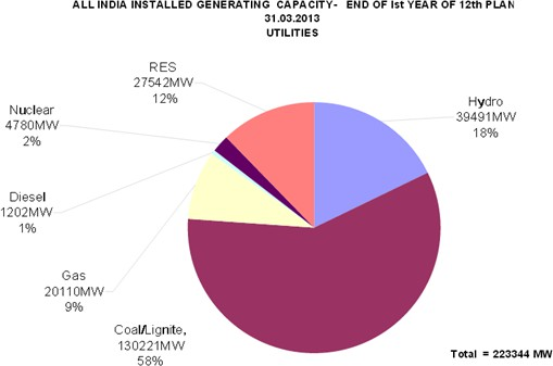
The power sector is one of the crucial inputs to the growth of industrial sectors and overall economic growth of India. Human progress has been linked to the increase of energy consumed per capita. India has fourth largest installed generating capacity in world but the per capita consumption of electricity is very low, owing to a huge gap between demand and supply of power. Traditionally the power sector was dominated by the public sector but has now been opened for competition from private players by the government sector.
The electricity sector in India had an installed capacity of 237.742 GW as of February 2014, the world’s fourth largest. Captive power plants generate an additional 39.375 GW. Non Renewable Power Plants constitute 87.55% of the installed capacity, and renewable power plants constitute the remaining 12.45% of total installed capacity.
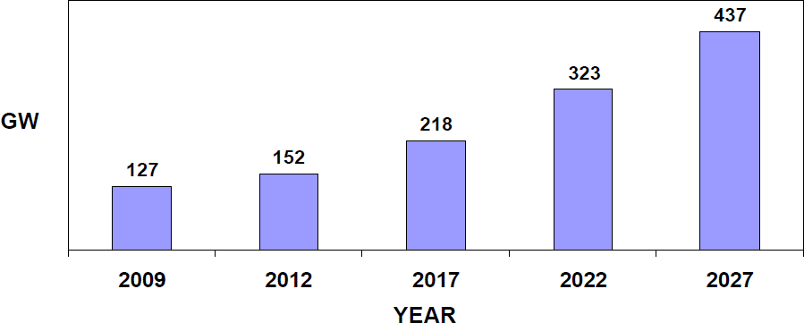
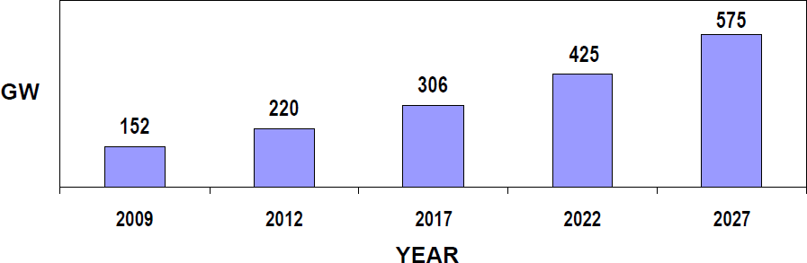
The projected Peak Demand in 2012 was about 150 GW and in 2017 is more than 200GW. The corresponding Installed capacity requirement in 2012 is about 220 GW and in 2017 is more than 300 GW. The projected Peak Demand and the Installed Capacity Requirement in next 15 years is shown in Fig.1.2 and 1.3 respectively.[31]
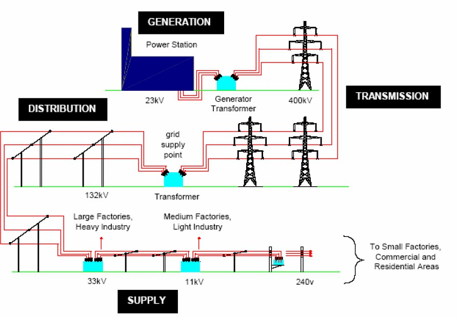
1.2 General structure of power system:
Power systems are comprised of 3 basic electrical subsystems.
- Generation subsystem
- Transmission subsystem
- Distribution subsystem
The sub-transmission system is also sometimes designated to indicate the portion of the overall system that interconnects the EHV and HV transmission system to the distribution system.
We distinguish between these various portions of the power system by voltage levels as follows:
- Generation:1kV-30 kV
- EHV Transmission: 500kV-765kV
- HV Transmission: 230kV-345kV
- Sub-transmission system: 69kV-169kV
- Distribution system: 120V-35kV
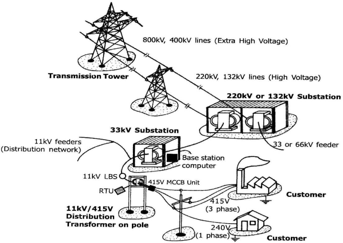
While transmission networks are built to transfer power from large generation units (over long distances) to the load areas, distribution networks are normally planned and built to distribute the power from the transmission network to the loads. Distribution networks can thus be considered as pure load supply networks.
1.3 Distribution systems:
Distribution systems serve as the link from the distribution substation to the customer. This system provides the safe and reliable transfer of electric energy to various customers throughout the service territory. Typical distribution systems begin as the medium- voltage three-phase circuit and terminate at a lower secondary three- or single-phase voltage typically below 1 kV at the customer’s premise, usually at the meter.
The distribution system is classified on the basis of voltage as
- Primary distribution systems (11 kV,6.6kV, 3kV)
- Secondary distribution systems (415 V/230 V)
Primary distribution system (11 kV,6.6kV, 3kV):
The part of the electrical-supply system existing between the distribution substations and the distribution transformers is called the primary system. This system operates at voltages somewhat higher than general utilization and handles large blocks of electrical energy than the average low voltages consumer uses. The voltage used for primary distribution depends upon the amount of power to be conveyed and the distance of the substation required to be fed. Due to economic considerations, primary distribution is carried out by 3 phase, 3 wire system.
Secondary distribution systems (415 V/230 V):
The secondary distribution system receives power from the secondary side of distribution transformers at low voltage and supplies power to various connected loads via service lines. The secondary distribution system is the final sub-system of the power system. This system includes the range of voltages at which the ultimate consumer utilizes the electrical energy. The secondary distribution employs 400/230 V, 3 phase, 4 wire system. The secondary distribution systems are generally of the radial type.
Distribution feeder circuits usually consist of overhead and underground circuits in a mix of branching laterals from the station to the various customers. The circuit is designed around various requirements such as required peak load, voltage, distance to customers, and other local conditions such as terrain, visual regulations, or customer requirements. These various branching laterals can be operated in a radial configuration or as a looped configuration, where two or more parts of the feeder are connected together usually through a normally open distribution switch. High-density urban areas are often connected in a complex distribution underground network providing a highly redundant and reliable means connecting to customers. Most three-phase systems are for larger loads such as commercial or industrial customers.
1.4 Requirements of customers
A considerable amount of effort is necessary to maintain an electric power supply within the limit for various types of consumers. Some of the requirements of distribution system are proper voltage, availability of power on demand and reliability.
- Voltage: One important requirement is that voltage variation at consumer’s terminals should be as low as possible. The changes in the voltage are due to the variation of load on the system. Low voltage cause loss of revenue, inefficient lighting and possible burningout of motors. High voltage causes lamps to burn out permanently and may cause failure of other appliances. Therefore a good distribution system should ensure that voltage variations at consumer terminals are within permissible limits. The statutory limits of voltage variation is +5% of the rated value at consumer terminals. Thus if the declared voltage is 11kV, the highest voltage of the consumer should not exceed 55kV while the lowest voltage of the consumer should not be less than 10.45kV.
- Availability of power on demand: Power must be available to the customers in any amount that they may require from time to time. For example motors may be started or shut down, lights may be turned on or off without prior notice to the electric supply company. As electrical energy cannot be stored therefore distribution system must be capable of supplying load demands of the consumers.
- Reliability: Modern industry is almost dependant on electric power for its operation. Homes and office buildings are lighted, heated or cooled and ventilated by electric This calls for reliable service.
2. LITERATURE SURVEY
2.1 Optimal sizing and siting of DG:
Electric power system development has been, for more than half a century, based on centralized large generating stations, with large generating units at a relatively small number of locations. In these stations, the voltage was stepped up to high voltage transmitted over long distances and again stepped down to low voltage and power was supplied to the customers. Over the last few years, electricity demand got larger as well as environmental concerns and the assessment of renewable energy resources as the source of cheap and domestic electricity generation has lead to the increased interest in the use of small-scale generation, connected to local distribution systems, which is commonly called Distributed Generation (DG). Environmental friendly electricity supply, electricity market liberalization, constraints on the construction of new transmission lines, increasing demand, highly reliable electricity supply, and reduction of the usage of fossil fuel resources are some of the reasons that are promoting the use of DG.
The use of DG is justified only when the planning of the power system with DG is done meticulously. Several factors are to be considered like proper sizing or capacity of distributed generation, number of such units, and its proper allocation in the power systems, types of generating unit etc. Among these factors, the problem of installation of DG units at proper location and sizing is of great importance. The selection of the best places for installation and the proper sizing of the DG units in large distribution systems is a complex combinatorial optimization problem. For the solution of these problems, several optimization techniques have been proposed in several research works.
Appropriate size and location of Distributed Generation (DG) plays a major role in minimizing power loss, improve the voltage profile and to improve the overall performance efficiency of distribution networks. Many researchers have proposed different methods to solve the above mentioned problems. For optimal allocation of DG in distribution networks, different objectives such as power loss minimization [2-16], improvement of voltage profile [2, 6, 14, 16], investment cost minimization [17, 18, 19], reduction of environmental impact [2], etc. were touched by the researchers using single or multi objective problem formulation. Different optimization techniques, like analytical approaches [5, 8-11, 14, 15, 20,], Genetic algorithm (GA) [19, 12, 15], Artificial bee colony [21], Particle swarm optimization [21], Evolutionary programming [13], Optimal power flow (OPF) [4], heuristic [18] and index based [2, 16] have been applied to solve the above DG allocation issues.
A methodology for optimal allocation of DG in distribution networks based on analytical approach (sensitivity analysis based on equivalent current injection) for loss reduction has been suggested by Gozel and Hocaoglu [5]. Wang and Nehrir [8] proposed an analytical method based on phasor current injection method to optimally place DG assuming uniformly, increasingly and centrally distributed load pattern within radial distribution network to minimize power loss.
Ghosh et.al.,[22] have used a simple conventional iterative search approach for determining optimal size and optimal placement of DG using Newton-Raphson (N-R) method of load flow study. The paper also focuses on optimization of weighting factor, which balances the cost and loss factors and it helps to build up desired objectives with maximum potential benefit. Borges C.L.T. and Falcão D.M.[23] have proposed a methodology of optimization process to optimize the allocation and sizing of DG units in order to minimize the electrical losses in primary distribution network and to guarantee acceptable reliability levels and voltage profile. The optimization problem is solved by the combination of genetic algorithm (GA) techniques with the methods to evaluate DG impacts in system reliability, losses and voltage profile, for optimal DG units allocation and sizing in order to maximize the benefit/cost relation, where the benefit is measured by the reduction of electrical losses and the cost is dependent on investment and operational cost incurred in their installation.
2.2 Optimization techniques:
As discussed above there are different analytical and evolutionary methods for optimization. Some of them are discussed below.
2.2.1 Classical methods:
The classical methods of optimization are useful in finding the optimum solution of continuous and differentiable functions. These methods are analytical and make use of the techniques of differential calculus in locating the optimum points. Since some of the practical problems involve objective functions that are not continuous and/or differentiable, the classical optimization techniques have limited scope in practical applications.
Some of the methods of optimization include:
- Linear programming: studies the case in which the objective function f is linear and the setA is specified using only linear equalities and (A is the design variable space)
- Integer programming: studies linear programs in which some or all variables are constrained to take on integer values.
- Quadratic programming:allows the objective function to have quadratic terms, while the set A must be specified with linear equalities and inequalities.
- Nonlinear programming: studies the general case in which the objective functionor the constraints or both contain nonlinear parts.
- Dynamic programming:studies the case in which the optimization strategy is based on splitting the problem into smaller sub-problems.
The difficulties associated with using mathematical optimization on large-scale engineering problems have contributed to the development of alternative solutions.
Linear programming and dynamic programming techniques, for example, often fail (or reach local optimum) in problems with large number of variables and non-linear objective functions [24].To overcome these problems, researchers have proposed evolutionary-based algorithms for searching near-optimum solutions to problems.
2.2.2 Evolutionary algorithms (EAs)
EAs are stochastic search methods that mimic the natural biological evolution and/or the social behavior of species. Such algorithms have been developed to arrive at near- optimum solutions to large-scale optimization problems, for which traditional mathematical techniques may fail. The five recent evolutionary-based algorithms: genetic algorithms, memetic algorithms, particle swarm, ant-colony systems, and shuffled frog leaping.
To mimic the efficient behavior of these species, various researchers have developed computational systems that seek fast and robust solutions to complex optimization problems.
· Genetic algorithm:
The first evolutionary-based technique introduced in the literature was the genetic algorithms (GAs) [25]. GA was developed based on the Darwinian principle of the ‘survival of the fittest’ and the natural process of evolution through reproduction. Based on its demonstrated ability to reach near-optimum solutions to large problems, the GAs technique has been used in many applications in science and engineering.
GA work with a random population of solutions (chromosomes). The fitness of each chromosome is determined by evaluating it against an objective function. To simulate the natural survival of the fittest process, best chromosomes exchange information (through crossover or mutation) to produce offspring chromosomes. The offspring solutions are then evaluated and used to evolve the population if they provide better solutions than weak population members. Usually, the process is continued for a large number of generations to obtain a best-fit (near optimum) solution. GA is explained in detail in chapter 5.
· Memetic algorithm(MA):
MAs are inspired by Dawkins’ notion of a meme [26], MAs are similar to GAs but the elements that form a chromosome are called memes, not genes. The unique aspect of the MAs algorithm is that all chromosomes and offspring are allowed to gain some experience, through a local search, before being involved in the evolutionary process [27]. Similar to the GAs, an initial population is created at random. Afterwards, a local search is performed on each population member to improve its experience and thus obtain a population of local optimum solutions. Then, crossover and mutation operators are applied, similar to GAs, to produce offspring. These offspring are then subjected to the local search so that local optimality is always maintained.
· Ant colony optimization(ACO) :
ACO was developed by Dorigo et al[28] based on the fact that ants are able to find the shortest route between their nest and a source of food. In the real world, ants (initially) wander randomly, and upon finding food return to their colony while laying down pheromone trails. If other ants find such a path, they are likely not to keep traveling at random, but instead follow the trail laid by earlier ants, returning and reinforcing it if they eventually find food. Over time, however, the pheromone trail starts to evaporate, thus reducing its attractive strength. The more time it takes for an ant to travel down the path and back again, the more time the pheromones have to evaporate. A short path, by comparison, gets marched over faster, and thus the pheromone density remains high .Pheromone evaporation has also the advantage of avoiding the convergence to a locally optimal solution. If there were no evaporation at all, the paths chosen by the first ants would tend to be excessively attractive to the following ones. In that case, the exploration of the solution space would be constrained. Thus, when one ant finds a good (short) path from the colony to a food source, other ants are more likely to follow that path, and such positive feedback eventually leaves all the ants following a single path. The idea of the ant colony algorithm is to mimic this behavior with “simulated ants” walking around the search
space representing the problem to be solved. . They have an advantage over simulated annealing and genetic algorithm approaches when the graph may change dynamically. The ant colony algorithm can be run continuously and can adapt to changes in real time.
· Particle swarm optimization(PSO):
PSO was introduced by Kennedy and Eberhart in 1995. It was inspired by the swarming behavior as is displayed by a flock of birds, a school of fish, or even human social behavior being influenced by other individuals. PSO consists of a swarm of particles moving in an n-dimensional, real-valued search space of possible problem solutions [29]. Every particle has a position vector encoding a candidate solution to the problem (similar to the genotype in EAs) and a velocity vector. Moreover, each particle contains a small memory that stores its own best position seen so far and a global best position obtained through communication with its neighbor particles. The process involves both social interaction and intelligence so that birds learn from their own experience (local search) and also from the experience of others around them (global search).
· Shuffled frog leaping algorithm(SFL):
The SFL algorithm, in essence, combines the benefits of the genetic-based MAs and the social behavior-based PSO algorithms. In the SFL [29], the population consists of a set of frogs (solutions) that is partitioned into subsets referred to as memeplexes. The different memeplexes are considered as different cultures of frogs, each performing a local search.Within each memeplex, the individual frogs hold ideas, that can be influenced by the ideas of other frogs, and evolve through a process of memetic evolution. After a defined number of memetic evolution steps, ideas are passed among memeplexes in a shuffling process. The local search and the shuffling processes continue until defined convergence criteria are satisfied.
· Simulated annealing (SA):
SA is a related global optimization technique that traverses the search space by testing random mutations on an individual solution. A mutation that increases fitness is always accepted. In SA parlance, one speaks of seeking the lowest energy instead of the maximum fitness. SA can also be used within a standard GA algorithm by starting with a relatively high rate of mutation and decreasing it over time along a given schedule.In the simulated annealing method, each point of the search space is compared to a state of some physical system, and the function to be minimized is interpreted as the internal energy of the system in that state. Therefore the goal is to bring the system, from an arbitrary initial state, to a state with the minimum possible energy
- DISTRIBUTEDGENERATION
Under the current centralized generation paradigm, electricity is mainly produced at large generation facilities, shipped though the transmission and distribution grids to the end consumers. However, the recent quest for energy efficiency and reliability led to explore possibilities to alter the current generation paradigm and increase its overall performances. In this context, one of the best candidates to complement the existing paradigm is distributed generation where electricity is produced next to its point of use.
3.1 Definition:
IEEE defines distributed generation as the ‘generation of electricity by facilities that are sufficiently smaller than central generating plants so as to allow interconnection at nearly any point in a power system.’
Distributed generation (or DG) generally refers to small-scale (typically 1 kW – 50 MW) electric power generators that produce electricity at a site close to customers or that are tied to an electric distribution system. Distributed generators include, but are not limited to synchronous generators, induction generators, reciprocating engines, micro turbines (combustion turbines that run on high-energy fossil fuels such as oil, propane, natural gas, gasoline or diesel), combustion gas turbines, fuel cells, solar photovoltaics, and wind turbines.
If small DG units are connected to the distribution network, the load is predominating and the power injection from the DG units will reduce the total network load. In such cases it is often possible to consider the DG units as negative loads.
3.2 Types of DG:
Some categories that define the size of the generation unit are presented in Table 3.1
Table 3.1: Types of DG
| Table 3.1: Types of DG | |
| Type | Size |
| Micro distributed generation | 1 Watt<5kW |
| Small distributed generation | 5kW< 5MW |
| Medium distributed generation | 5MW < 50MW |
| Large distributed generation | 50MW <300MW |
The DGs can be grouped into four major types based on terminal characteristics in terms of real and reactive power delivering capability.
You can download the Project files here: Download files now. (You must be logged in).
· Type1: DG delivering only P
This type DG is capable of delivering only active power such as photovoltaic, micro- turbines, fuel cells, which are integrated to the main grid with the help of converters/inverters.The photovoltaics are elaborated further:
Photovoltaic System:
Photovoltaic system has been increasingly used in medium sized grid with domestic utilities. PV panels are connected in series and parallel to generate usable amount of voltage and current. By series connection voltage level can be built up and by parallel connection current density can be increased.
In photovoltaic systems, a grid connected inverter converts the DC output voltage of the solar modules into the AC system. The grid-connected photovoltaic (PV) system extracts maximum power from the PV arrays. The maximum power point tracking (MPPT) technique is usually associated with a DC-DC converter. The DC-AC injects the sinusoidal current to the grid and controls the power factor.
Type2: DG delivering both P & Q
This type of DG is capable of delivering both active and reactive power. DG units based on synchronous machines (cogeneration, gas turbine, etc.) come under this type.
Synchronous Generators: The synchronous generator is the absolutely dominating generator type in power systems. It can generate active and reactive power independently and has an important role in voltage control. The synchronizing torques between generators act to keep large power systems together and make all generator rotors rotate synchronously.
For high power, the electrically excited type is employed. For medium and low power the permanent magnet synchronous machine is used or hybrid excited type, i.e. both permanent magnet and electrically field generation systems are used in correlation. In cases of electrically excited generators, when the machine is over-excited it injects reactive power into the grid.
· Type3: DG delivering only Q
These types of DGs are capable of delivering only reactive power. Synchronous compensators such as gas turbines are the example of this type and operate at zero power factors.
Synchronous condenser (sometimes called a synchronous capacitor or synchronous compensator) is a device identical to synchronous motor, a shaft is not connected to anything but spin freely. Its purpose is not to convert electric power to mechanical power or vice versa, but to adjust conditions on the electric power transmission grid. Its field is controlled by a voltage regulator to either generate or absorb reactive power as needed to adjust the grid’s voltage, or to improve power factor. The condenser’s installation and operation are identical to large electric motors.
Increasing the field excitation of the device results in its furnishing reactive power (VARs) to the system. Its principal advantage is the ease with which the amount of correction can be adjusted. The kinetic energy stored in the rotor of the machine can help stabilize a power system during short circuits or rapidly fluctuating loads such as electric arc furnaces. Large installations of synchronous condensers are sometimes used in association with high-voltage direct current converter stations to supply reactive power to the alternating current grid.
Unlike a capacitor bank, the amount of reactive power from a synchronous condenser can be continuously adjusted. Reactive power from a capacitor bank decreases when grid voltage decreases, while a synchronous condenser can increase reactive current as voltage decreases. However, synchronous machines have higher energy losses than static capacitor banks. Most synchronous condensers connected to electrical grids are rated between 20 Mvar(Megavars) and 200 Mvar and many are hydrogen cooled.
· Type4:DG delivering P and consuming Q
These types of DG are capable of delivering active power but consuming reactive power. Mainly induction generators, which are used in wind farms, come under this category. However, doubly fed induction generator (DFIG) systems may consume or produce reactive power i.e. operates similar to synchronous generator.
Doubly Fed Induction Generators (DFIG):
Doubly-fed induction generators (DFIGs) are by far the most widely used type of
doubly-fed electric machine, and are one of the most common types of generator used to produce electricity in wind turbines. Doubly-fed electric machines are basically electric machines that are fed ac currents into both the stator and the rotor windings. Most doubly-fed electric machines in industry today are three-phase wound-rotor induction machines.
The primary advantage of doubly-fed induction generators when used in wind turbines is that they allow the amplitude and frequency of their output voltages to be maintained at a constant value, no matter the speed of the wind blowing on the wind turbine rotor. Because of this, doubly-fed induction generators can be directly connected to the ac power network and remain synchronized at all times with the ac power network. Other advantages include the ability to control the power factor (e.g., to maintain the power factor at unity), while keeping the power electronics devices in the wind turbine at a moderate size.
3.3 Advantages of distributed generation:
- Flexibility – DG resources can be located at numerous locations within a utility’s service This aspect of DG equipment provides a utility tremendous flexibility to match generation resources to system needs.
- Improved Reliability – DG facilities can improve grid reliability by placing additional generation capacitycloser to the load, thereby minimizing impacts from transmission and distribution (T&D) system disturbances, and reducing peak- period congestion on the local grid. Furthermore, multiple units at a site can increase reliability by dispersing the capacity across several units instead of a single large central plant. .
- Reduced Loading of T&D Equipment – By locating generating units on the low- voltage bus of existing distribution substations, DG will reduce loadings on substation power transformers during peak hours, therebyextending the useful life of this equipment and deferring planned substation upgrades
- Reduces the necessity to build new transmission and distribution lines or upgrade existing ones.
- Reduce transmission and distribution line losses [1]
- Improve power quality and voltage profile of the system.[1] DG can serve as a cost effective alternative to major system upgrades for peak shaving or enhancing load capacity margins. Additionally, if the needed generation facilities could be constructed to meet the growing demand, the entire distribution and transmission system would also require upgrading to handle the additional loading.
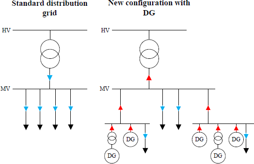
3.4 Impact of DG:
The power system faces many problems when distributed generation is added in the already existing system; this is because the power system is not designed with distributed generation in mind. The addition of generation could influence power quality problems, degradation in system reliability, reduction in the efficiency, over voltages and safety issues. On the other side the power system distribution are well designed which could handle the addition of generation if there is proper grounding, transformers and protection is provided. But there are limits to the addition of distributed generations if it goes beyond its limit then it is important to modify and change the already designed distributed system equipment and protection, which could in a result facilitate the integration of new generation.
The connections of renewable and distributed generation to distribution networks have increased complexity in the existing network operation and regulation. Such difficulty is mainly due to a transformation of the network from passive to become more active where new generation is being connected. As a consequence, there have been a number of technical and non-technical impacts being experienced in the distribution networks.
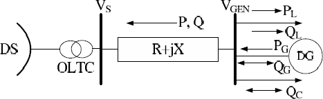
- Voltage rise at the DG connection point is the most significant impact for the network operators. At the points moving away from the substation, lines or cablestend to have smaller cross-sectional area. This indicates that the line resistance becomes larger (lines are highly resistive); therefore, the ratio between the line reactance and resistance (X/R ratio) is smaller. As a consequence, active power flow has more influence on voltage change than reactive power, i.e., the first term associated with active power and line resistance. Therefore, the increased power exports from DG can potentially cause voltage rise at the point of connection.
- Reverse Power Flow: Distribution networks were historically designed to distribute power in one direction, i.e., fromHV transmission systems to lower voltage
networks. The connections of DG to distribution networks can result in a reverse of power flows. This occurs when the generation produced is more than local load in the system. A surplus of power is therefore exported to a higher voltage system to supply the demand elsewhere in the grid.
- Power Quality: Power quality issues in a distribution network mainly comprise voltage flicker and harmonics.The connection of variable DG can be a potential cause of voltage flicker. Harmonics arise from the presence of harmonic components from non-linear devices such as power supplies, compact fluorescent lights, variable speed motor drives, inverter-coupled generators and power factor correction capacitors that can absorb or inject current into the system. These current-led harmonic components will cause distortion of voltage waveform of the supply from an ideal sinusoidal shape at 50 Hz at higher frequencies. The major adverse effects of harmonic distortion include heating of induction motors, transformers and capacitors. However, recent innovations in power electronics such as fast switching, high voltage Insulated Gate Bipolar Transistors (IGBT) and developments in power generation technologies have made DG a considerable alternative.
· Protection :
Penetration of a DG into an existing distribution system has many impacts on the system, with the power system protection being one of the major issues. DG causes the system to lose its radial power flow, besides the increased fault level of the system caused by the interconnection of the DG. Short circuit power of a distribution system changes when its state changes. Short circuit power also changes when some of the generators in the distribution system are disconnected. This may result in elongation of fault clearing time and hence disconnection of equipments in the distribution system or unnecessary operation of protective devices.
The most common configuration in distribution systems is radial. In this type of configurations only one source feeds a downstream network. Therefore on a radial system without DG, the relay protection will see downstream faults because only in that direction will appear power flow. In this situation the fault is cleared opening the breaker of the main feeder because only the main feeder can contribute to the fault. When DG is present in the system, an additional power flow appears from load side to source side and vice versa, therefore the opening of the main feeder breaker does not assure that the fault is cleared.
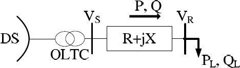
- POWERFLOW OF RADIAL DISTRIBUTION SYSTEM
4.1 Backward forward sweep method
Power flow analysis is an important and efficient tool to know the real and reactive power losses in the system. Implementation of accurate, efficient and fast method of power flow analysis forms the base for the study of radial distribution system (RDS) with DG.The power flow analysis also determines the line flow in each line section in kW and the power loss in each section.
The variables for the power flow analysis of distribution system are different from that of transmission system. This is because distribution network is radial in nature having high R/X ratios, where as transmission system is loop in nature having high X/R ratio .Hence, the conventional Gauss-Seidel and Newton Raphson method do not converge for distribution networks.
There exist a number of algorithms for the power flow studies. The efficiency of such power flow algorithm is of utmost importance as each optimization study requires numerous power flow runs. Backward/Forward sweep (BFS) methods [30] take the advantage of the radial nature and have become the preferred method for distribution systems.
As a distribution feeder is radial, iterative techniques commonly used in transmission network power-flow studies are not used because of poor convergence characteristics. Instead, an iterative technique specifically designed for a radial system is used.
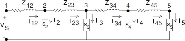
For the nonlinear ladder network shown above it is assumed that all of the line impedances and load impedances are known along with the voltage at the source (Vs).
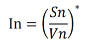
The load current at each node is computed by:
For this end node case, the line current I45 is equal to the load current I5. Applying
Kirchhoff’s voltage law (KVL), the voltage at Node 4 (V4) can be determined:
V4 = V5 + Z45*I45
The load current I4 can be determined, and then Kirchhoff’s current law (KCL) applied to determine the line current I34.
I34 = I45 + I4
Kirchhoff’s voltage law is applied to determine the node voltage V3 .This procedure is continued until a voltage (V1) has been computed at the source. The first iteration will produce a voltage that is not equal to the specified source voltage Vs. Because the network is nonlinear, multiplying currents and voltages by the ratio of the specified voltage to the computed voltage will not give the solution. The most direct modification to the ladder network theory is to perform a backward sweep. The backward sweep commences by using the specified source voltage and the line currents from the forward sweep. Kirchhoff’s voltage law is used to compute the voltage at Node 2 by:
V2 = VS – Z12*I12
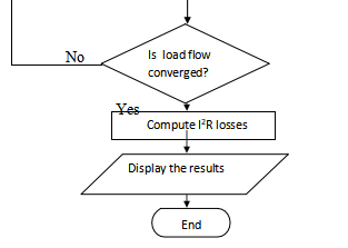
This procedure is repeated for each line segment until a new voltage is determined at Node 5. Using the new voltage at Node 5, a second forward sweep is started that will lead to a new computed voltage at the source. The power is calculated using S=V*I. The forward and backward sweep process is continued until the difference between the successive power values is within a given tolerance.
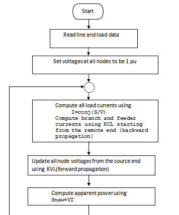
The flowchart for the forward backward sweep method is as follows:
5. OPTIMAL SITING AND SIZING OF DISTRIBUTED GENERATION IN RADIAL DISTRIBUTION SYSTEM
5.1 Problem formulation:
As stated earlier the planning of electric system with the presence of DG requires several factors to be taken into account such as the number and capacity of the units, best location etc. Hence the problem of DG allocation is of great importance. The use of an optimization method for selection of best places for installation and size of DG units in large distribution systems is a complex optimization problem. Genetic algorithms offer a new and powerful approach to these optimization problems.
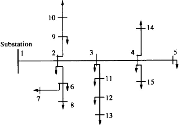
We have considered the following standard 15 bus radial distribution system. The details of the system are given in appendix I.
You can download the Project files here: Download files now. (You must be logged in).
5.1.1 Objective function:
The main goal of the proposed algorithm is to determine the best locations for new distributed generation resources by minimizing different functions. The following objectives are considered:
- Loss
- Voltage profile
- Cost
5.2 Genetic algorithm
- Genetic algorithm: A concept
The first evolutionary-based technique introduced in the literature was the genetic algorithms (GAs) .Genetic algorithm (GA) is a search technique used in computing to find true or approximate solutions to optimization and search problems. Genetic algorithms are search algorithms based on the mechanics of natural selection and natural genetics. They combine survival of the fittest string structures with a structured yet randomized information exchange to form a search algorithm with some of the innovative flair of human search. GA allows a population composed of many individuals to evolve under specified selection rules to a state that maximizes the “fitness” (i.e., minimizes the cost function).
There are four basic operations within Genetic Algorithms they are evaluation, selection, crossover and mutation [32,33].
The general flowchart for this technique is as follows:
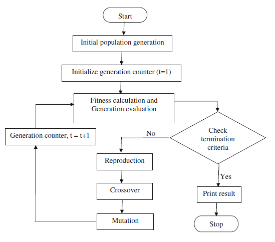
5.3 Methodology:
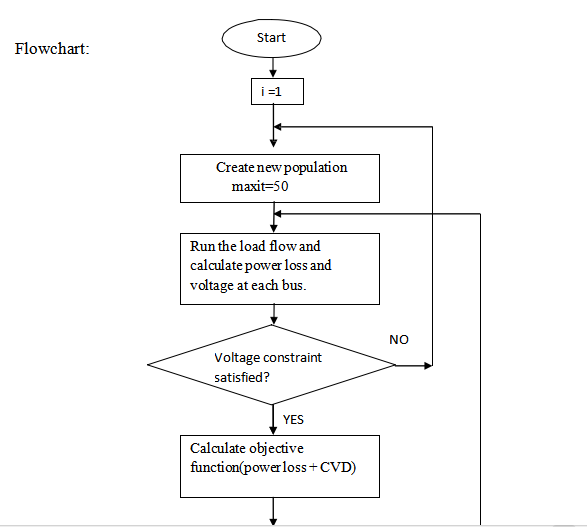
As discussed earlier, the optimal sizing and location of DG is a complex optimization problem. Genetic algorithm (GA) is used as a tool to solve this problem. The initial population size is 32 i.e. we have 32 probable solutions. The size of chromosome (each member of the population) is 8 bits, first 4 bits indicate location or the bus number and next 4 bits indicate size of the DG.GA program along with the power flow is executed according to the steps described in the last section with constraints for:
- Voltage: The voltage variations must be within ± 5% of the rated
- Power loss: When DG is connected the power loss must be less than the case when DG is not connected.
- Busat which DG is connected: The DG should not be connected at bus no 1 and
The stopping criterion for GA is the number of iterations (maxit) which we can specify.
The power flow program is according to the backward forward sweep (BFS) method in which we have used the power mismatch method.
The line and load data for the 15 bus system (Annexure I) is referred for this program. This program is defined as function and is called in the main program for GA as and when required. The inputs passed to this function are the bus number and the size of the DG. This subroutine then returns the value of voltage, losses which are further used for analysis in the program for GA. The DG is considered as negative load.
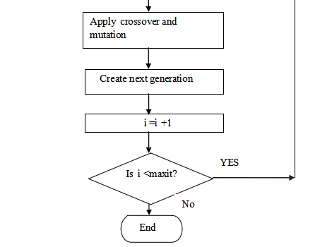
The GA sorts the fitness function according its values and gives the best result. The flowchart for genetic algorithm for distributed generation is as follows:
6. RESULTS
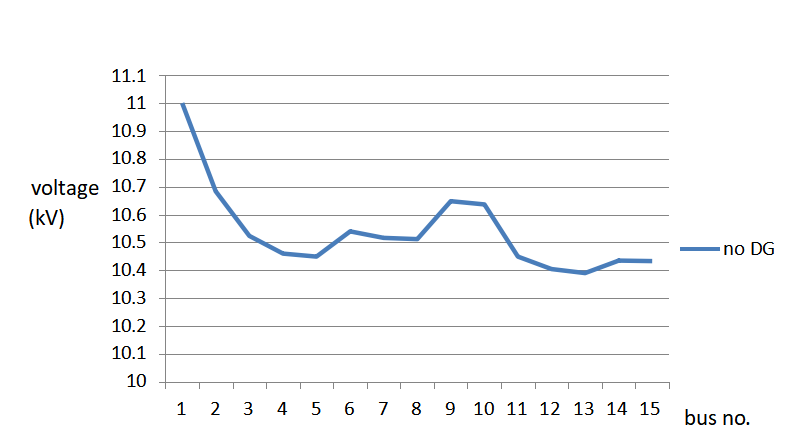
6.1. Voltage profile of 15 bus radial distribution system without DG
For radial distribution systems, unidirectional power flow from the substations to the customers can be assumed. The highest voltage can be expected at the substations whereas the lowest voltage occurs at the customer points of connection. Hence, the voltage is decreasing from the substation along the feeders to the customers.
Table 6.1: Voltages at various buses of 15-bus distribution system
| Bus no. | Voltages(in kV) |
| 1 | 11 |
| 2 | 10.684 |
| 3 | 10.5233 |
| 4 | 10.4599 |
| 5 | 10.449 |
| 6 | 10.5403 |
| 7 | 10.5159 |
| 8 | 10.5122 |
| 9 | 10.6476 |
| 10 | 10.6358 |
| 11 | 10.4494 |
| 12 | 10.404 |
| 13 | 10.3896 |
| 14 | 10.4346 |
| 15 | 10.433 |
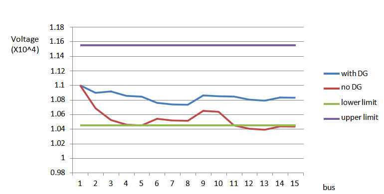
6.2 Impact of Addition of DG on Voltage Profile and losses
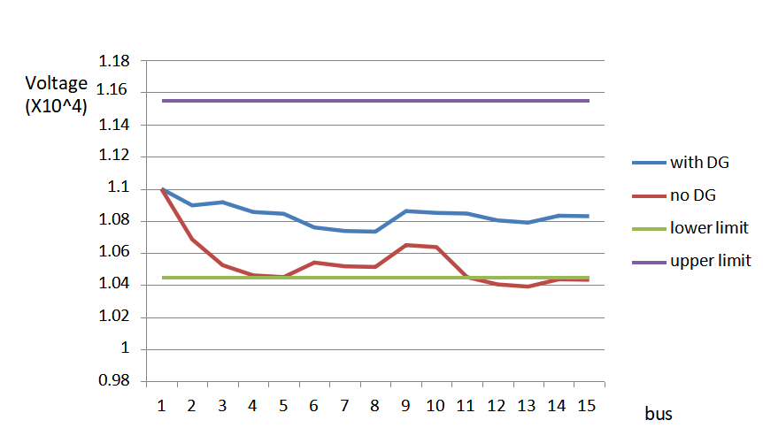
6.2.1 Effect on voltage profile
When DG is connected in the distribution system, the voltages at all the nodes improve. Also, there is considerable reduction in losses as can be seen in the table below.
Table 6.2 Effect of addition of DG on losses
| Size of DG added | 1 MW at 0.85 pf |
| Location of DG | 3 |
| Losses with DG | |
| Losses without DG | 62.12 kW |
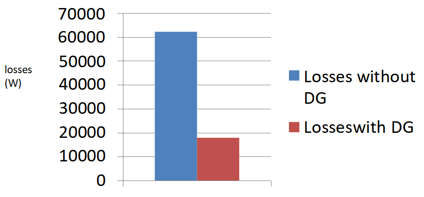
6.2.2 Saving in losses
DG of size 1 MW at 0.85 pf is connected at bus no. 3 and the losses are computed using power flow method.
| Losses with DG | 17.86 kW |
| Losses without DG | 62.12 kW |
You can download the Project files here: Download files now. (You must be logged in).
Power injections from DGs change network power flows thereby modifying energy losses. Electrical line loss occurs when current flows through transmission and distribution systems. The magnitude of the loss depends upon amount of current flow and line resistance. Therefore, line loss can be decreased by reducing either line current or resistance or both. If DG is used to provide energy locally to the load, the line loss can be reduced because of decrease in current flow in some part of the network.
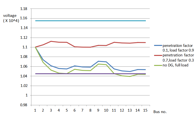
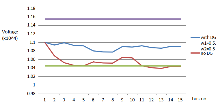
6.3 Comparison of voltage profiles considering worst case scenarios
Voltage violations due to presence of distributed generators can considerably limit the amount of power supplied by these generators in distribution networks. Before installing (or allowing the installation of) a distributed generator, utility engineers must analyze the worst operating scenarios to guarantee that the network voltages will not be adversely affected by the generators. These scenarios are characterized by the following:
- No generation and maximum demand;
- Maximum generation and minimum demand;
- Minimum generation and maximum
Voltage profile for the 3 cases is as follows:
Table 6.3 Voltage profile considering worst case scenarios
| Bus no. | Voltage (kV) | ||
| No DG | Penetration factor=0.1 Load factor=0.9 | Penetration factor=0.7 Load factor=0.3 | |
| 1 | 11.0000 | 11.0000 | 11.0000 |
| 2 | 10.6840 | 10.7380 | 11.0470 |
| 3 | 10.5230 | 10.6130 | 11.1200 |
| 4 | 10.4600 | 10.5560 | 11.1020 |
| 5 | 10.4490 | 10.5470 | 11.0990 |
| 6 | 10.5400 | 10.6100 | 11.0060 |
| 7 | 10.5160 | 10.5880 | 10.9990 |
| 8 | 10.5120 | 10.5850 | 10.9980 |
| 9 | 10.6480 | 10.7060 | 11.0360 |
| 10 | 10.6360 | 10.6950 | 11.0330 |
| 11 | 10.4490 | 10.5470 | 11.0990 |
| 12 | 10.4040 | 10.5060 | 11.0860 |
| 13 | 10.3900 | 10.4940 | 11.0820 |
| 14 | 10.4350 | 10.5340 | 11.0950 |
| 15 | 10.4330 | 10.5320 | 11.0940 |
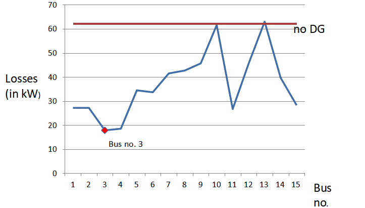
6.4 Calculation of losses after connecting DG of a particular size at all nodes.
Connecting DG of 1 MW at each bus, the losses are computed using the power flow program. Minimum losses are observed at bus no. 3.
| Size of DG considered | 1 MW at 0.85 pf |
| Optimum bus location | 3 |
6.5 Impact of size on power loss
Distribution networks were historically designed to distribute power in one direction, i.e. from HV transmission systems to lower voltage networks. The connections of DG to distribution networks can result in a reverse of power flows. This occurs when the generation produced is more than local load in the system. A surplus of power is therefore exported to a higher voltage system to supply the demand elsewhere in the grid.
Total connected load = (1.226 + 1.25j) * 106
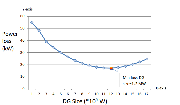
Results show energy loss variation as a function of the DG penetration level. It presents a characteristic U-shape trajectory. Losses start to decrease with increasing DG penetration levels, whereas after a minimum value of power loss, they start to increase with higher DG penetration levels.
6.6 Effect of placement of DG at non-optimal location
If DG units are connected at non-optimal locations, the system losses may increase, thus resulting in increased costs. Studies have indicated that inappropriate locations or sizes of DG may lead to greater system losses than the ones in the existing network. Hence both, sizing and siting, are necessary.
Table 6.4 Effect of placement of DG at non-optimal location
| Size of DG connected | 1.2 MW at 0.85 pf |
| Bus at which DG is connected | 13 |
| Losses without DG | 62.12 kW |
| Losses with DG | 82.82 kW |
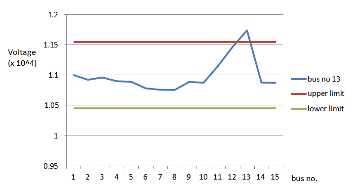
From the above figure, it can be seen that when DG is connected at a non-optimal location the losses are greater than when DG is not connected.
Also, the voltage may exceed the 5% voltage limit. Hence, adding power loss and voltage constraints is necessary.
For finding the optimum size and location an evolutionary algorithm technique Genetic Algorithm is used.
6.7 Optimum sizing and siting using Genetic Algorithm
Genetic Algorithm is used for obtaining optimum size and location of DG. The following results are obtained.
| Size of DG obtained | 1 MW at 0.85 pf |
| Location of DG | 3 |
| Losses with DG | 17.081 kW |
| Losses without DG | 62.12 kW |
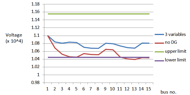
6.7.1 3 objectives
Objectives: 1) Losses
- CVD
- Cost
(Assumption: Cost is considered as a linear function of size)
Table 6.9 Voltage profile with 3 objectives: losses, CVD, cost
| Bus no. | Without DG (kV) | With DG (kV) |
| 1 | 11.0000 | 11.0000 |
| 2 | 10.6840 | 10.8370 |
| 3 | 10.5230 | 10.8040 |
| 4 | 10.4600 | 10.8300 |
| 5 | 10.4490 | 10.8200 |
| 6 | 10.5400 | 10.7000 |
| 7 | 10.5160 | 10.6760 |
| 8 | 10.5120 | 10.6730 |
| 9 | 10.6480 | 10.8020 |
| 10 | 10.6360 | 10.7900 |
| 11 | 10.4490 | 10.7340 |
| 12 | 10.4040 | 10.6910 |
| 13 | 10.3900 | 10.6780 |
| 14 | 10.4350 | 10.8060 |
| 15 | 10.4330 | 10.8040 |
Table 6.10 Results for 3-objective function
| Size of DG connected | 700 kW at 0.85 pf |
| Location of DG | 4 |
| Losses with DG | 21.83 kW |
| Losses without DG | 62.12 kW |
| Vmin | 10.67 kV |
| Vmax | 11 kV |
| CVD | 0.084 |
You can download the Project files here: Download files now. (You must be logged in).
6.8 Voltage profile and losses for different types of DG
Genetic algorithm along with load flow is executed and the following results are obtained.
When different types of DGs are connected, the following optimal location, size and voltage profiles are obtained.
Total connected load= (1.23 + 1.25j) * 106
- Types of DG
Table 6.11 Different types of DG
| Type | Size (x106) | Location | Losses |
| P + jQ | 1.2+0.74 j | 3 | 17.08 kW |
| P – jQ | 0.4 – 0.25 j | 2 | 54.89 kW |
| P | 1 | 3 | 35.98 kW |
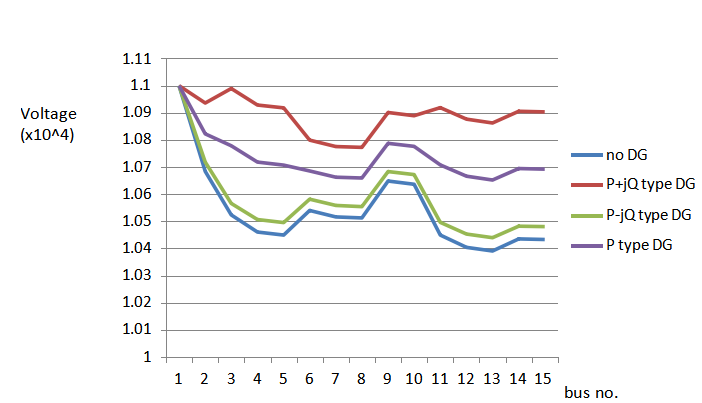
It can be observed that P + jQ type DG, as compared to others, has significant influence on quantities such as:
- Real power loss reduction;
- Improved voltage
Hence, we have considered P+jQ type of DG for our analysis.
6.9 Convergence of Genetic Algorithm
6.9.1. Convergence of GA for multi-objective function: 2 objectives: losses and CVD
GA for 2 objective function: losses and CVD converges in 3 iterations as can be seen from the plot.
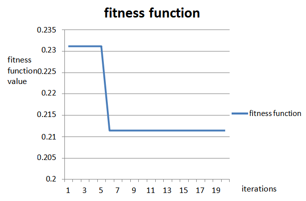
6.9.2 Convergence of Genetic Algorithm with iterations
GA initially considers a random population i.e. a random 8 bit chromosome representing size and location. The load flow calculates the losses, CVD and population get sorted according to value of fitness function. The best cases are kept for next iterations and the remaining cases are replaced by new cases after performing crossover and mutation. With every iteration, the solution moves towards the best solution.
For multi-objective function with 2 variables: losses and CVD Population size=16
No. of iterations=20
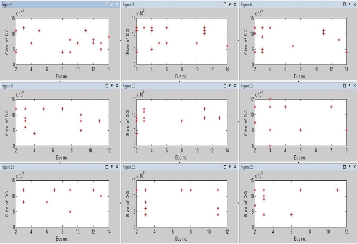
Plots obtained for size vs location for few cases are compared in figure 6.13.
Here, the optimum solution is obtained at bus no. 3, where the size of DG to be placed is
1.2 MW at 0.85 pf. This value is obtained in the 6th iteration as can be seen from figure 6.10 and 6.13.
In the further iterations, the points move towards this solution.
7. CONCLUSION
In conclusion, the power flow analysis for the standard 15-bus radial distribution system was successfully developed using the backward/forward sweep (BFS) method, which served as the foundation for studying the impact of distributed generation (DG). The results clearly showed that the size and location of DG units significantly influence system performance, particularly in terms of losses and voltage profile. Improper allocation of DG can lead to higher losses and increased operational costs, highlighting the importance of optimization in DG planning. To address this, a Genetic Algorithm (GA), an evolutionary optimization technique, was applied to determine the optimal size and location of DG units. The study demonstrated that the GA-based approach effectively minimized system losses and improved voltage profiles under both single-objective and multi-objective scenarios. Furthermore, when cost was incorporated alongside losses and cumulative voltage deviation (CVD), the optimal DG placement strategy shifted, emphasizing the need to consider economic as well as technical factors in decision-making. Overall, the proposed method provides an efficient and practical solution for optimal DG allocation and sizing in radial distribution systems.
REFERENCES
- Acharya, P. Mahat, and N. Mithulananthan, “An analytical approach for DG allocation in primary distribution network,” International Journal of Electrical Power & Energy Systems, vol. 28, no. 10, pp 669- 678, Dec. 2006.
- Chiradeja and R. Ramkumar, “An approach to quantify the technical benefits of distributed generation”, IEEE Trans on Energy Conversion, vol. 19, no. 4, pp.764-773, December 2004
- H. Mendez Quezeda, Jua-Rivier Abbad, and T.Gomez, “Assessment of energy distribution losses for increasing penetration of DG”, IEEE Trans on Power Systems, vol. 21, no. 2, pp. 533-540, May 2006.
- F. Ochoa and G. P. Harrison, “Minimizing energy losses: Optimal accommodation and Smart operation of renewable DG”, IEEE Trans on Power Systems, vol. 26, no. 1, pp. 198-205, February 2011.
- Gozel and M. H. Hocaoglu, “An Analytical method for the Sizing and Siting of Distributed Generators in Radial System”, International Journal of ElectricPower System Research, vol. 79, no. 6, pp. 912-918, June 2009.
- H. Hedayati, S. A. Nabaviniaki, and Adel Akbarimazd, “A method for placement of DG units in distribution network”, IEEE Trans on Power Delivery, vol. 23, no. 3, pp. 1620-1628, July 2008.
- M. Atwa, E. F EI-Saadany, M. M. A. Salama, and R. Seethapathy, “Optimal renewable resource mix for distribution system energy loss minimization”, IEEE Trans on Power Systems, vol. 25, no. 1, pp. 360-370, February 2010.
- Wang and M. H. Nehir, “Analytical approach for optimal placement of distributed generation sources in power system”, IEEE Trans on Power Systems, vol. 19, no. 4, pp. 2068-2076, November 2004.
- Acharya, P. Mahat, and N. Mithulananthan, “An analytical approach for DG allocation in primary distribution network”, Electrical Power and Energy Systems, vol. 28, pp. 669–678, 2006.
- Q. Hung, N. Mithulananthan, and R. C. Bansal, “Analytical expressions for DG allocation in primary distribution networks”, IEEE Trans on Energy Conversion, vol. 25, no. 3, September 2010.
- Q. Hung, N. Mithulanathan, and R. C. Bansal, “Multiple distributed generators placement in primary distribution networks for loss reduction”, IEEE Trans on Industrial Electronics, vol. 60, no. 4, pp. 1700-1708, April 2013.
- Mithulanathan, Than Oo, and Lee Van Phu, “Distributed generator placement in power distribution system using Genetic Algorithm to reduce losses”, Thammasat Int. J. Sc. Tech., vol. 9, no. 3, pp. 55-62,2004.
- K. Khatod, V. Pant, and J. D.Sharma, “Evolutionary programming based optimal placement of renewable distributed generators”, IEEE Trans on Power Systems, 99, pp. 1-13, 2012.
- Khan and M. A. Choudhary, “Implementation of distributed generation (IDG) algorithm for performance enhancement of distribution feeder under extreme load growth”, Electric Power and Energy Systems, no. 32, pp. 985-997, 2010.
- N. Shukla, S. P. Singh, V. Srinivas Rao, and K. B. Naik, “Optimal sizing of distributed Generation placed on radial distribution systems”, Electric Power Components and Systems, no. 38, pp. 260-274, 2010.]
- H. Mendez, J. Rivier, J. I. De la Fuente, T. Gomez et al., “Impact of distributed generation on distribution investment deferral”, International Journal of Electrical Power and Energy Systems, vol. 28, no. 4, pp. 244–252,May 2006.
- Giani Celli, Emilio Ghiani, Susanna Mocci, and Fabrizio Pilo, “A multi- objective evolutionary algorithm for siting and sizing of distributed generation”, IEEE Trans on Power Systems, vol. 20, no. 2, pp. 750-757, May2005.]
- L. Willis, “Analytical methods and rules of thumb for modelling DG distribution interaction,” in proc. IEEE Power Engineering Society summer meeting, vol. 3, pp.1643-1644, 2000.
- S. Abu-Mouti and M. E. El-Hawary, “Optimal distributed generation allocation and sizing in distribution systems using artificial bee colony algorithm”, IEEE Trans on Power Delivery, vol. 26, no. 4, pp. 2090-2101,October 2011.
- EI-Khattam, K. Bhattacharya, Y. G. Hagazy, and M. M. A. Salama, “Optimal investment planning for distributed generation in a competitive electricity market”,IEEE Trans on Power Systems, vol. 9, no. 3, pp. 1674-1684, August 2004.
- Sudipta Ghosh, S.P. Ghoshal and Saradindu Ghosh. “Optimal sizing and placement of distributed generation in a network system”, Electrical Power and Energy Systems 32 (2010): 849-856.]
- Gopiya Naik, D. K. Khatod, and M. P. Sharma, “Optimal allocation of distributed generation in distribution system for loss reduction”, International conference on product development and renewable energy resources (ICPDRE 2012), Coimbatore (India). pp. 42-46, 2012.
- Carmen L.T. Borges, Djalma M. Falcão. “Optimal distributed generation allocation for reliability, losses, and voltage improvement”, Electrical Power and Energy Systems 28 (2006): 413-420
- Lovbjerg M. Improving particle swarm optimization by hybridization of search heuristics and self-organized criticality. Masters Thesis, Aarhus University, Denmark; 2002.
- Holland J. Adaptation in natural and artificial systems. Ann Arbor, MI: University of Michigan Press, 1975.
- Dawkins The selfish gene. Oxford: Oxford University Press; 1976.
- Merz P, Freisleben B. A genetic local search approach to the quadratic assignment problem. In: Ba¨ck CT, editor. Proceedings of the 7thinternational conference on genetic algorithms. San Diego, CA:Morgan Kaufmann; 1997. p. 465–72.
- Dorigo M,Maniezzo V,ColorniA.Ant system: optimization by a colony of cooperating agents. IEEE Trans SystMan Cybern 1996;26(1):29–41.
- Emad Elbeltagi, Tarek Hegazy, Donald Grierson, “Comparison among five evolutionary-basedoptimization algorithms”, Advanced Engineering Informatics 19 (2005)
- K. Krishna Murthy, Dr. S.V. Jaya Ram Kumar “Three-Phase Unbalanced Radial Distribution Load Flow Method”, Internationally referred journal of engineering and science(IRJES) , Volume1 Issue ,1 September 2012.
- “Transmission and distribution in India”, Report published by Power Grid Corporation of India ltd PGCIL.
- Randy Haupt, Sue Ellen Haupt, ‘Practical Genetic Algorithms’, John Wiley and sons, Inc., Publication
- K.F. Man, K.S.Tang, and S. Kwong, “Genetic Algorithms: Concepts and Applications”, IEEE Transactions on Industrial Electronics, Vol. 43, No. 5, Oct. 1996.
You can download the Project files here: Download files now. (You must be logged in).
Keywords: Optimal siting of distributed generation, optimal sizing of distributed generation, radial distribution system, genetic algorithm optimization, backward forward sweep load flow, active power loss minimization, voltage profile improvement, multi-objective function, renewable energy integration, distribution system reliability.


Responses