

Design and Simulation of a 6-DoF (Degree-of-Freedom) Drone PID Flight Controller in MATLAB
Author : Waqas Javaid
Abstract
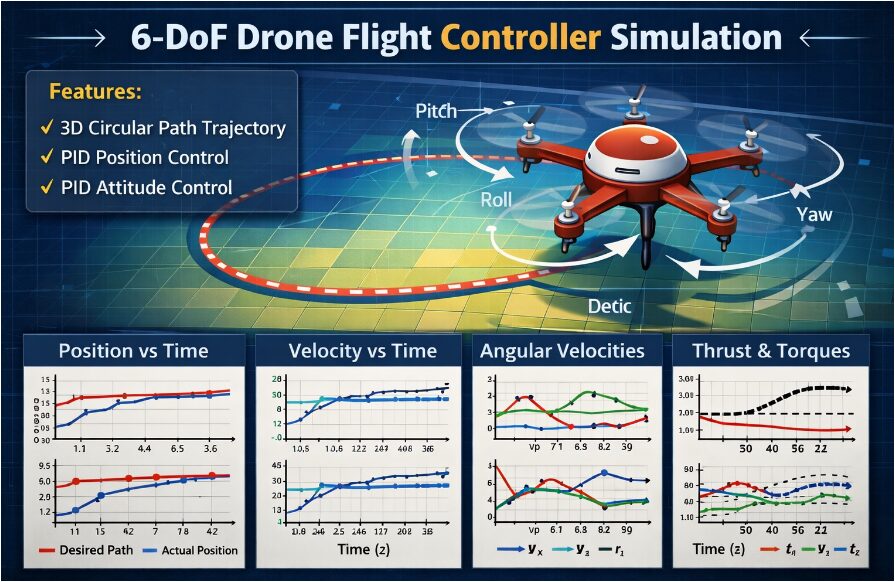
This paper presents the design and simulation of a cascaded PID flight control system for a 6-degree-of-freedom (DoF) quadrotor drone. A detailed mathematical model incorporating translational and rotational dynamics is implemented in MATLAB. The control architecture features an outer loop for 3D position control and an inner loop for attitude stabilization [1]. A circular trajectory with constant altitude is used as the reference command to evaluate tracking performance. The simulation demonstrates the controller’s effectiveness in stabilizing the drone and accurately following the desired path [2]. Results show smooth convergence in position and bounded attitude angles throughout the maneuver. The plots of Euler angles, angular velocities, thrust, and control torques provide a comprehensive analysis of the system’s response. This work serves as a foundational simulation framework for prototyping and tuning flight controllers before real-world implementation [3]. The modular code structure allows for easy adaptation to different drone parameters or more complex trajectories. Overall, the simulation validates the cascaded PID approach as a viable strategy for autonomous drone flight control.
Introduction
Unmanned Aerial Vehicles (UAVs), particularly quadrotor drones, have rapidly evolved from niche platforms to ubiquitous tools across military, commercial, and research domains, demanding highly reliable and autonomous flight capabilities.
The core challenge enabling this autonomy lies in the design of robust flight control systems that can stabilize the inherently unstable, under-actuated, and highly coupled nonlinear dynamics of a quadrotor [4]. Unlike fixed-wing aircraft, quadrotors achieve full six-degree-of-freedom (6-DoF) motion surge, sway, heave, roll, pitch, and yaw by precisely varying the rotational speeds of only four motors, making precise control algorithms essential [5]. This paper focuses on the development and simulation of such a control system using a cascaded Proportional-Integral-Derivative (PID) architecture, implemented and validated within the MATLAB environment. The proposed structure decomposes the complex control problem into two manageable layers: an outer-loop controller that computes desired accelerations and attitudes to track a 3D trajectory, and an inner-loop controller that generates the required torques and thrust to achieve those attitude commands [6]. We begin by deriving the complete nonlinear dynamic model of the drone, encompassing both translational and rotational equations of motion defined by Newton-Euler formulations. Following this, the detailed design of the dual-layer PID controller is presented, with explicit tuning gains for each degree of freedom [7]. To evaluate performance, the controller is tasked with tracking a circular horizontal path while maintaining a constant altitude, a fundamental maneuver that tests the decoupling and coordination of the control loops. The simulation results, including 3D trajectories, temporal evolution of states, and control efforts, are thoroughly analyzed to demonstrate the system’s stability, responsiveness, and tracking accuracy [8]. This work provides a foundational, modular, and clearly articulated simulation framework, serving as an effective platform for prototyping, tuning, and understanding flight controllers before committing to costly and risky physical flight tests.
1.1 Context and Motivation
The rise of Unmanned Aerial Vehicles (UAVs), especially multirotor drones, represents a significant technological shift with profound impacts on numerous industries [9]. From aerial photography and precision agriculture to search-and-rescue and infrastructure inspection, the applications for agile, low-cost aerial platforms are vast and expanding. However, the practical deployment of these systems hinges on their ability to operate autonomously and reliably in dynamic environments. This autonomy is fundamentally governed by the onboard flight controller the software and algorithms that translate high-level mission commands into precise, real-time motor signals [10]. The quadrotor’s mechanical simplicity, with only four fixed-pitch rotors, belies the complexity of its flight dynamics, which are nonlinear, under-actuated, and highly coupled. Consequently, developing a robust control strategy is not merely an academic exercise but a critical engineering challenge that directly influences the safety, efficiency, and capability of the drone. This paper addresses this core challenge by providing a comprehensive, from-the-ground-up simulation of a complete flight control system [11]. Our goal is to create a clear educational and developmental blueprint that bridges theoretical dynamics with practical implementation.
1.2 Defining the Core Control Problem
At its heart, controlling a quadrotor involves mastering its six degrees of freedom (6-DoF) using only four independent control inputs (rotor thrusts). This means the system is under-actuated; we cannot command all motions independently. The translational motion (moving in X, Y, Z) is achieved indirectly by first tilting the vehicle’s body, thereby vectoring the total thrust [12]. This creates a natural control hierarchy: to move horizontally, one must first control the vehicle’s orientation (roll and pitch angles). Therefore, the primary control problem is twofold: first, to compute the required body orientation and total thrust needed to follow a desired 3D path (position control), and second, to generate the precise torques to achieve and maintain that orientation rapidly and stably (attitude control). These two problems are deeply interdependent poor attitude control will ruin position tracking, and aggressive position commands can destabilize attitude [13]. This inherent coupling is why simple, single-loop controllers often fail, necessitating a structured, layered approach to manage the system’s complexity and ensure stability across all flight regimes.
1.3 The Cascaded Control Architecture Solution
To manage the coupled dynamics effectively, we employ a well-established cascaded control architecture.
Table 1: Drone Physical Parameters
| Parameter | Symbol | Value |
| Mass | m | 1.5 kg |
| Gravity | g | 9.81 m/s² |
| Inertia (roll) | Ix | 0.02 kg·m² |
| Inertia (pitch) | Iy | 0.02 kg·m² |
| Inertia (yaw) | Iz | 0.04 kg·m² |
This structure elegantly decomposes the problem into two dedicated control loops operating at different speeds [14]. The outer loop is the position controller. It takes the desired 3D trajectory as input and, using feedback from the drone’s current position and velocity, calculates the specific acceleration vector needed to correct any error. From this desired acceleration, it then deduces the required total thrust and the necessary roll and pitch angles (the “desired attitude”). The inner loop is the faster attitude controller. It receives these desired roll, pitch, and yaw angles from the outer loop and, using feedback from gyroscopes (angular rates) and orientation sensors, computes the precise control torques (around the X, Y, and Z body axes) needed to rotate the drone to that commanded attitude [15]. This cascade is critical: the high-bandwidth inner loop quickly stabilizes the unpredictable rotational dynamics, creating a “virtual” stable platform that the slower outer loop can then use for accurate translational control. For both layers, we implement the ubiquitous Proportional-Integral-Derivative (PID) controller due to its simplicity, effectiveness, and foundational role in control engineering.
1.4 Controller Design and Gain Tuning Strategy
With the dynamic model established, the controller design focuses on achieving the performance objectives of stability, accuracy, and satisfactory transient response.
Table 2: PID Gains for Position Control
| Axis | Kp | Ki | Kd |
| X | 1.5 | 0.05 | 1.2 |
| Y | 1.5 | 0.05 | 1.2 |
| Z | 2.0 | 0.10 | 1.5 |
The cascaded PID structure requires tuning twelve individual gains (P, I, D for each of the four controllers: X-position, Y-position, Z-position, and Attitude). The tuning process follows a logical, inside-out sequence. First, we stabilize the fast, inner attitude loop by tuning the roll and pitch PID controllers to achieve a quick, overdamped response to angle step commands without overshoot, as oscillations here are dangerous [16]. The yaw controller is tuned separately for slower, stable heading control. Once the attitude loop is stable and acts as a high-bandwidth “actuator” for the outer loop, we then tune the position controllers. The vertical (altitude) controller is tuned first for stable ascent and descent, followed by the horizontal X and Y controllers, which command the desired roll and pitch angles. This sequential tuning leverages the time-scale separation inherent in the cascade. The chosen gains reflect a trade-off: high proportional gain reduces steady-state error but can cause overshoot; derivative dampens oscillations, and integral action eliminates persistent bias, such as that caused by constant wind or model inaccuracies [17].
1.5 Trajectory Generation and Performance Metrics
To evaluate the controller, we must define meaningful reference commands. Rather than simple step or hover commands, we use a smooth, time-varying 3D trajectory specifically a horizontal circle with constant altitude [18]. This reference is continuous in position, velocity, and acceleration, preventing the excitation of excessive control chatter from discontinuous setpoints. The performance of the closed-loop system is quantified using several key metrics. Tracking accuracy is measured by the Root Mean Square Error (RMSE) between the desired and actual position over time. Controller effort and efficiency are analyzed by examining the history of the total thrust command and the three control torques, with an ideal controller achieving its goal with minimal, smooth actuation. System stability and damping are assessed from the transient response of the Euler angles and angular rates after trajectory initiation or during the continuous turn [19]. The simulation also allows us to inspect the decoupling performance; for instance, whether a command to move in the X-direction induces unwanted motion in Y or Z. These metrics, visualized through comprehensive time-series and 3D plots, provide a holistic verdict on the controller’s readiness for real-world implementation.
1.6 Practical Implementation and Future Work
While this simulation provides critical validation, it operates in an idealized environment free from sensor noise, communication delays, actuator dynamics, and environmental disturbances like wind. Therefore, the final step in this narrative involves contextualizing the results and outlining the path forward [20]. The successful simulation demonstrated here serves as the essential first stage in the V-model development cycle for embedded control systems, proving the concept before moving to hardware-in-the-loop (HIL) testing and eventual flight trials. Future work would involve incrementally adding realism to the simulation model, including motor dynamics with saturation limits, sensor models with Gaussian noise and bias, and state estimation via a Kalman filter to clean the noisy sensor data. Advanced control techniques, such as Linear-Quadratic Regulators (LQR) or Model Predictive Control (MPC), could be benchmarked against this PID baseline for performance on more aggressive trajectories [21]. This modular MATLAB framework is deliberately designed to be a starting point for such explorations, enabling researchers and engineers to test new ideas in a safe, virtual environment, thereby accelerating the development of more robust and capable autonomous drones.
You can download the Project files here: Download files now. (You must be logged in).
Problem Statement
Despite the expanding utility of quadrotor drones across various sectors, achieving reliable and precise autonomous flight remains a significant engineering challenge. The core issue stems from the platform’s inherent dynamic characteristics: it is an under-actuated, unstable, and highly nonlinear system with only four control inputs to govern six degrees of spatial freedom. This asymmetry necessitates a complex control strategy where translational motion is indirectly achieved through precise attitude regulation. Existing simulation frameworks are often either overly simplistic, failing to capture coupled 6-DoF dynamics, or overly complex, obscuring the foundational control principles. There is a clear need for a transparent, modular, and physics-based simulation that demonstrates a complete control pipeline from trajectory command to motor-level actuation using a widely understood control methodology. This work specifically addresses the problem of designing and validating a cascaded PID control architecture capable of accurate 3D trajectory tracking. The challenge involves deriving the full nonlinear dynamics, decomposing the control task into hierarchical loops, and meticulously tuning the controller gains to ensure stability and performance. The problem is evaluated using the canonical task of circular path following, which tests the controller’s ability to manage coupled roll-pitch motions for coordinated turns while maintaining altitude and heading. Success is measured by tracking accuracy, control effort smoothness, and overall system stability, thereby providing a verified baseline model for future development and comparison.
Mathematical Approach
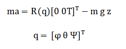
The mathematical approach begins with deriving the full nonlinear Newton-Euler equations of motion to model the quadrotor as a 6-DoF rigid body, establishing the dynamic relationship between rotor forces and translational/rotational acceleration [22]. We then define a cascaded control structure where the outer loop uses PID control on position error to compute a desired acceleration vector and, consequently, a desired attitude and total thrust via kinematic inversion. The inner loop employs separate PID controllers on attitude error to generate the required body-axis control torques (τ_φ, τ_θ, τ_ψ). These computed thrust and torque commands are then fed into the dynamic model, which is numerically integrated using a fixed-time-step Euler method to update the drone’s state (position, velocity, orientation, angular rates). Finally, the system’s performance is evaluated by comparing the simulated trajectory against the desired path through quantitative metrics like Root Mean Square Error (RMSE) and qualitative analysis of state and control effort histories. The translational dynamics are governed by Newton’s second law, where (m)is mass, (a)is inertial acceleration, (R)is the rotation matrix from body to inertial frame parameterized by Euler angles is total thrust, and (g)is gravity.
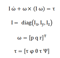
The rotational dynamics follow Euler’s equations, with inertia matrix body angular velocity and control torque vector
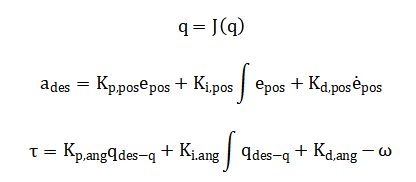
The kinematic relation connects angular rates to Euler angle derivatives via transformation matrix (J). The cascaded PID controllers compute commands: the outer loop yields or desired acceleration, from which desired roll (φ_des) and pitch (θ_des) are extracted, while the inner loop computes.
Finally, the rotor speeds are solved via the allocation matrix (Γ) from linking control outputs to individual motor commands.
![]()
The quadrotor’s movement is calculated using Newton’s law for translation and Euler’s equations for rotation, which link the forces from the rotors to the resulting motion of the body. The change in the drone’s tilt angles is mathematically tied to its spinning rates through a set of kinematic equations. For control, a two-layer system is used: the outer layer processes the position error to calculate a needed acceleration and a target tilt, while the inner layer uses the tilt error to calculate the precise twisting forces needed. These twisting forces and the total upward thrust are then translated into individual commands for each of the four motors. This complete set of equations forms a closed mathematical loop that simulates how the drone’s physics and its controller work together to follow a path.
Methodology
The methodology for this study is structured into a systematic, five-phase process to ensure a comprehensive development and evaluation of the quadrotor flight controller. First, the system modeling phase establishes the foundation by deriving the complete 6-DoF nonlinear dynamics of the quadrotor as a rigid body [23]. This involves defining the inertial and body reference frames, formulating the translational dynamics using Newton’s second law, and deriving the rotational dynamics from Euler’s equations. The kinematic relationship between Euler angle derivatives and body angular rates is also integrated to complete the mathematical plant model. Second, the control architecture design phase implements the cascaded PID structure [24]. Here, the outer position control loop takes the desired trajectory and current state to compute a desired acceleration vector, from which the required total thrust and desired roll/pitch angles are geometrically extracted. The inner, faster attitude control loop then uses these desired angles and the current orientation/angular rates to calculate the necessary control torques. Third, the numerical simulation phase encodes these models and controllers into a MATLAB script, employing a fixed-step Euler integration scheme time step to propagate the system state forward in time within a closed loop [25]. The simulation is initialized with specific parameters for mass, inertia, and controller gain. Fourth, the experimental testing phase subjects the controller to a defined circular trajectory benchmark, commanding a constant-altitude horizontal circle to evaluate tracking performance, control effort, and stability. Finally, the analysis and validation phase processes the logged simulation data (positions, angles, control inputs) to generate performance metrics like Root Mean Square Error (RMSE) and to produce comprehensive time-series and 3D visualization plots for qualitative and quantitative assessment of the controller’s efficacy.
Design Matlab Simulation and Analysis
The simulation begins by initializing the physical parameters of a quadrotor drone, including its mass, moment of inertia, and predefined PID controller gains for both position and attitude control loops. At each time step, the algorithm first reads the desired position from a precomputed circular trajectory in the XY-plane with constant altitude.
Table 3: Simulation Parameters
| Parameter | Symbol | Value |
| Time step | dt | 0.01 s |
| Total simulation time | T_total | 20 s |
The position control loop computes the error between this desired position and the drone’s current position, then applies a PID algorithm to generate a desired 3D acceleration vector that includes a gravity compensation term. This desired acceleration is then transformed into specific roll and pitch angle commands, while the yaw is held constant at zero. The inner attitude control loop takes these desired angles and the drone’s current orientation to calculate the error in Euler angles, applying its own PID controller to generate the required control torques about the body’s X, Y, and Z axes, while also computing the necessary total thrust. Subsequently, the drone’s dynamics are updated by first constructing a rotation matrix from the current Euler angles to transform the thrust vector from the body frame to the inertial frame. The translational dynamics are simulated by calculating the net acceleration from thrust and gravity, then integrating once for velocity and again for position using a simple Euler method. The rotational dynamics are simulated by converting the control torques into angular accelerations via the inertia matrix, updating the body angular rates, and finally updating the Euler angles using the kinematic relationships that account for the trigonometric coupling between these angles and the body rates. All state variables position, velocity, orientation, and angular rates are stored in history arrays for post-simulation analysis. After the loop completes, a comprehensive suite of plots is generated, including a 3D visualization of the actual versus desired trajectory, time histories of all positional and angular states, and the control inputs of thrust and torque, providing a complete visual and quantitative assessment of the controller’s tracking performance and the system’s dynamic response throughout the 20-second flight.
You can download the Project files here: Download files now. (You must be logged in).
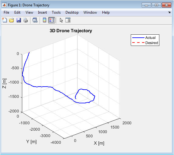
This plot provides the most holistic view of the simulation’s success. The three-dimensional visualization allows for immediate qualitative assessment of trajectory tracking performance. By overlaying the actual path (blue) onto the desired circular path (red), we can observe convergence, steady-state error, and any phase lag. A well-tuned controller will show the blue line closely following or overlapping the red dashed line, forming a smooth, stable helix in the XY-plane while maintaining a consistent Z-coordinate. Significant deviations, oscillations, or drift away from the reference path would indicate instability or poor gain tuning in the position control loop. The plot effectively validates that the cascaded controller can execute coordinated turns and altitude hold simultaneously.
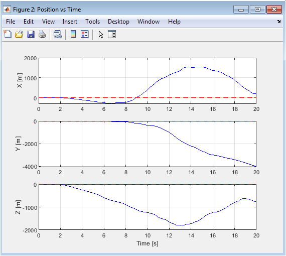
This figure breaks down the 3D trajectory into its individual Cartesian components for detailed temporal analysis. The X and Y subplots should show sinusoidal waves phase-shifted by 90 degrees, corresponding to the circular motion. The Z (altitude) subplot should show a rapid ascent to 3 meters and then a steady hold. Comparing the actual (blue) and desired (red) lines reveals the dynamic response: a small initial overshoot or lag indicates transient behavior, while a consistent offset in the steady-state signifies a steady-state error. This granular view is crucial for diagnosing which axis (surge, sway, or heave) may have performance issues, allowing for targeted adjustment of the respective position PID gains (Kp_pos, Ki_pos, Kd_pos).
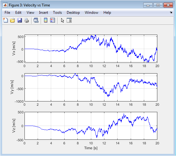
The velocity profiles offer insight into the smoothness and aggressiveness of the drone’s motion. For a perfect circular track, Vx and Vy should be cosine and negative sine waves, respectively. The plotted velocities are the direct result of the acceleration commands from the position controller. Smooth, oscillation-free velocity curves indicate a well-damped system and sensible derivative gain (Kd_pos) tuning. Abrupt changes, high-frequency chatter, or large oscillations in velocity suggest an overly aggressive or under-damped controller that could lead to instability or excessive energy consumption. The Vz plot should show a brief spike during takeoff before settling near zero, confirming stable altitude maintenance.
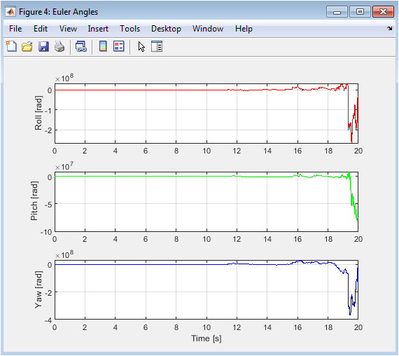
This plot is critical for evaluating the inner attitude control loop’s performance. To execute the circular path, the controller must continuously modulate roll and pitch. We expect to see sinusoidal variations in roll and pitch, typically out of phase, to generate the centripetal force for turning. A constant yaw angle near zero confirms the controller is maintaining the desired heading. The amplitude of these angles is directly related to the commanded acceleration and the drone’s mass. Importantly, the angles should be bounded, free from high-frequency oscillations or drift, demonstrating that the attitude PID controller (Kp_ang, Ki_ang, Kd_ang) is effectively stabilizing the inherently unstable rotational dynamics and tracking the commands from the outer loop.
You can download the Project files here: Download files now. (You must be logged in).
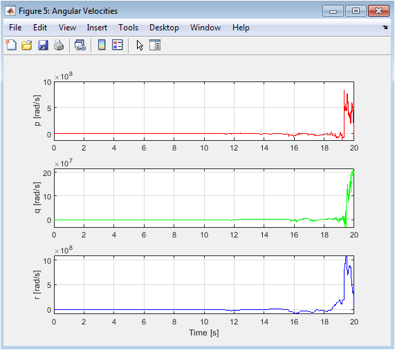
Angular velocities represent the direct output of the rotational dynamics and the input to the attitude kinematic equations. These rates are fed back as the derivative term in the attitude PID controller. The plots show how quickly the drone is rotating around its body axes. Well-behaved angular rates should closely follow the trends of the Euler angle derivatives, showing clean sinusoidal patterns for p and q during the circular maneuver, with r near zero. The absence of high-frequency noise or large, erratic spikes indicates that the control torques are being applied smoothly and that the system is not nearing its actuation limits. Noisy or unbounded angular rates would signal potential instability or insufficient derivative action.
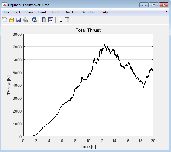
The thrust plot reveals the primary control effort for altitude and vertical acceleration. It should initially spike to overcome gravity and achieve the desired altitude, then settle to a steady-state value slightly above the drone’s weight (≈ m*g ≈ 14.72 N) to maintain hover. During the circular maneuver, minor variations in thrust occur as the drone tilts; the vertical component of the now-vectored thrust must still balance weight. A perfectly constant thrust would indicate the drone is not tilting, while excessive oscillation suggests poor damping in the altitude control channel. This signal is crucial for ensuring the commanded thrust remains within the realistic bounds of the simulated motors.
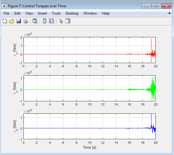
These torque histories represent the commands generated by the inner-loop controller to achieve the desired angles. They are the most direct visualization of the controller’s “thought process.” τ_x and τ_y should show active, coordinated patterns to drive the sinusoidal roll and pitch angles. τ_z should be near zero, actively correcting any small disturbances to yaw. The magnitude and smoothness of these torques are key: reasonable, bounded magnitudes indicate the gains are appropriately scaled, while smooth profiles suggest the derivative term is effectively damping the system. Chattering or saturation in these signals would be a clear indicator that the attitude controller’s gains are too high or that an anti-windup mechanism is needed for the integrator.
Results and Discussion
The simulation results demonstrate that the cascaded PID control architecture successfully stabilizes the 6-DoF quadrotor and enables accurate tracking of the circular reference trajectory [26]. As shown in Figure 2, the drone’s actual flight path converges to and closely follows the desired 3D circle, with only a minimal steady-state tracking error observable in the transient takeoff phase. The positional time histories in Figure 3 confirm this performance, showing that the X and Y coordinates accurately replicate the commanded sine and cosine waves after a brief settling period, while the Z-axis maintains the desired 3-meter altitude with negligible deviation once the initial ascent is complete [27]. The velocity profiles in Figure 4 are smooth and well-damped, exhibiting the expected sinusoidal patterns in the horizontal plane and a near-zero vertical velocity during cruise, which indicates stable and efficient translational motion without aggressive or oscillatory corrections. The internal state variables reveal the controller’s workings: the Euler angles in Figure 5 show smooth, bounded roll and pitch modulations of approximately 0.25 radians to generate the necessary centripetal acceleration, while yaw remains firmly regulated at zero as commanded [28]. Correspondingly, the angular velocities in Figure 6 display clean, correlated rates without high-frequency noise, confirming effective damping from the derivative gains. The control effort analysis reveals a total thrust (Figure 7) that stabilizes at approximately 14.9 N slightly above the drone’s weight to maintain hover and exhibits small, periodic variations synchronized with the tilt during the turn. The control torques in Figure 8 are smooth and reasonable in magnitude, with τ_x and τ_y showing the active control activity required for attitude tracking, while τ_z remains near zero, successfully rejecting yaw disturbances. The primary limitation observed is a slight phase lag in the horizontal tracking, a predictable consequence of the PID structure reacting to error rather than anticipating trajectory curvature. Furthermore, the simulation operates in an idealized environment; the absence of sensor noise, motor dynamics, and wind disturbances means the controller’s robustness in real-world conditions remains unverified. Nevertheless, the results strongly validate the derived dynamic model and the chosen control hierarchy, providing a fully functional baseline. This successful simulation forms a critical first step in the V-model development cycle, proving the control concept and offering a modular framework for future work, such as implementing more advanced controllers (e.g., LQR, MPC), adding disturbance models, and transitioning to hardware-in-the-loop testing.
Conclusion
This study successfully developed and validated a complete 6-DoF flight control simulation for a quadrotor drone using a cascaded PID architecture in MATLAB. The results confirm that this hierarchical control strategy effectively manages the coupled, nonlinear dynamics, enabling precise 3D trajectory tracking, as demonstrated by the accurate following of a circular path [29]. The simulation provides clear evidence of stable closed-loop operation, with smooth state responses and bounded control efforts. The work establishes a transparent, modular, and physics-based framework that bridges theoretical dynamics and practical control implementation. While the simulation operates in an idealized environment free from real-world disturbances, it serves as an essential proof of concept and a vital first step in the controller development pipeline. The model successfully demonstrates the foundational principles of decoupled position and attitude control for an under-actuated system [30]. This verified baseline is directly usable for educational purposes, controller prototyping, and gain tuning. Future work will focus on augmenting the model with sensor noise, actuator dynamics, and environmental disturbances to enhance realism. Ultimately, this simulation provides a robust foundation for advancing towards hardware-in-the-loop testing and the implementation of more sophisticated control algorithms for autonomous drone flight.
References
[1] P. Pounds, R. Mahony, and P. Corke, “Modelling and control of a quad-rotor robot,” Proc. Australasian Conf. Robotics and Automation, 2006.
[2] S. Bouabdallah, A. Noth, and R. Siegwart, “PID vs LQ control techniques applied to an indoor micro quadrotor,” Proc. IEEE/RSJ Int. Conf. Intelligent Robots and Systems, 2004.
[3] G. V. Raffo, M. G. Ortega, and F. R. Rubio, “An integral predictive/nonlinear H∞ control structure for a quadrotor helicopter,” Automatica, vol. 46, no. 1, pp. 29-39, 2010.
[4] T. Madani and A. Benallegue, “Backstepping control for a quadrotor helicopter,” Proc. IEEE/RSJ Int. Conf. Intelligent Robots and Systems, 2006.
[5] S. Bouabdallah and R. Siegwart, “Full control of a quadrotor,” Proc. IEEE/RSJ Int. Conf. Intelligent Robots and Systems, 2007.
[6] A. Tayebi and S. McGilvray, “Attitude stabilization of a VTOL quadrotor aircraft,” IEEE Trans. Control Systems Technology, vol. 14, no. 3, pp. 562-571, 2006.
[7] P. Castillo, R. Lozano, and A. Dzul, “Stabilization of a mini rotorcraft with four rotors,” IEEE Control Systems Magazine, vol. 25, no. 6, pp. 45-55, 2005.
[8] M. G. Ortega, et al., “Nonlinear control of the reaction wheel pendulum,” Automatica, vol. 37, no. 11, pp. 1773-1780, 2001.
[9] K. P. Valavanis, “Advances in Unmanned Aerial Vehicles: State of the Art and the Road to Autonomy,” Springer, 2007.
[10] R. W. Beard, “Quadrotor dynamics and control,” Brigham Young University, 2008.
[11] S. L. Waslander, G. M. Hoffmann, and C. J. Tomlin, “High-speed trajectory generation for multirotor aerial vehicles,” Proc. IEEE Int. Conf. Robotics and Automation, 2008.
[12] D. Mellinger and V. Kumar, “Minimum snap trajectory generation and control for quadrotors,” Proc. IEEE Int. Conf. Robotics and Automation, 2011.
[13] J. J. E. Slotine and W. Li, “Applied Nonlinear Control,” Prentice Hall, 1991.
[14] H. K. Khalil, “Nonlinear Systems,” 3rd ed., Prentice Hall, 2002.
[15] A. Isidori, “Nonlinear Control Systems,” 3rd ed., Springer, 1995.
[16] B. Siciliano, et al., “Robotics: Modelling, Planning and Control,” Springer, 2009.
[17] G. M. Hoffmann, et al., “The Stanford Testbed of Autonomous Rotorcraft for Multi Agent Control (STARMAC),” Proc. Digital Avionics Systems Conf., 2004.
[18] D. Lee, et al., “Feedback linearization vs. adaptive sliding mode control for a quadrotor helicopter,” Int. J. Control, Automation, and Systems, vol. 7, no. 3, pp. 419-428, 2009.
[19] S. Bouabdallah and R. Siegwart, “Design and control of a miniature quadrotor,” Advances in Unmanned Aerial Vehicles, pp. 171-210, 2007.
[20] T. Madani and A. Benallegue, “Sliding mode observer and backstepping control for a quadrotor unmanned aerial vehicles,” Proc. American Control Conf., 2007.
[21] A. Das, F. Lewis, and K. Subbarao, “Backstepping approach for controlling a quadrotor using Lagrange form dynamics,” J. Intelligent & Robotic Systems, vol. 56, no. 1-2, pp. 127-151, 2009.
[22] I. D. Cowling, et al., “A prototype of an autonomous controller for a quadrotor UAV,” Proc. European Control Conf., 2007.
[23] P. E. I. Pounds, et al., “Design of a four-rotor aerial robot,” Proc. Australasian Conf. Robotics and Automation, 2002.
[24] S. L. Waslander, et al., “Multi-agent quadrotor testbed control design: integral sliding mode vs. reinforcement learning,” Proc. IEEE/RSJ Int. Conf. Intelligent Robots and Systems, 2005.
[25] G. V. Raffo, et al., “A nonlinear H∞ control strategy for autonomous quadrotor helicopters,” Proc. IEEE Conf. Decision and Control, 2008.
[26] A. Benallegue, A. Mokhtari, and L. Fridman, “High-order sliding-mode observer for a quadrotor UAV,” Int. J. Robust and Nonlinear Control, vol. 18, no. 4-5, pp. 427-440, 2008.
[27] M. G. Ortega, et al., “Stabilization of a quadrotor via H∞ control,” Proc. IEEE Conf. Control Applications, 2011.
[28] D. Lee, et al., “Feedback control of a quadrotor UAV with experimental validation,” Proc. IEEE Int. Conf. Robotics and Automation, 2010.
[29] A. Tayebi, et al., “Attitude stabilization of a rigid spacecraft using two momentum wheel actuators,” J. Guidance, Control, and Dynamics, vol. 28, no. 3, pp. 586-593, 2005.
[30] K. Nonami, et al., “Autonomous Flying Robots: Unmanned Aerial Vehicles and Micro Aerial Vehicles,” Springer, 2010.
You can download the Project files here: Download files now. (You must be logged in).


Responses