

3D Molecular Dynamics Simulation with Velocity Verlet Algorithm in MATLAB
Author : Waqas Javaid
Abstract
This Molecular Dynamics simulation models the motion of 64 particles in a cubic box with periodic boundary conditions using reduced Lennard-Jones units. Particles interact via the Lennard-Jones potential truncated at a cutoff distance of 2.5σ, and their trajectories are integrated using the Velocity Verlet algorithm over 5000 time steps. Initial positions are arranged on a simple cubic lattice, while velocities are randomly assigned and scaled to achieve a reduced temperature of 1.0. The simulation computes kinetic, potential, and total energies, along with instantaneous temperature, to monitor system equilibrium [1]. Mean squared displacement is calculated from initial positions to track particle diffusion. The radial distribution function is generated by binning interparticle distances to characterize structural order. Output visualizations include energy and temperature trends, MSD, RDF, a 3D snapshot of final positions, and a histogram of velocity magnitudes [2]. The code demonstrates core principles of molecular dynamics including neighbor interactions, periodic boundary conditions, and statistical ensemble averaging. This framework can be extended for larger systems, different ensembles, or more complex potentials in advanced simulations [3].
Introduction
Molecular Dynamics (MD) simulation is a powerful computational technique used to study the physical movements and interactions of atoms and molecules over time, providing a bridge between microscopic behavior and macroscopic observables.
This method integrates Newton’s equations of motion for a system of interacting particles, allowing researchers to investigate thermodynamic, structural, and transport properties from first principles. In reduced Lennard-Jones units, the simulation becomes particularly elegant as it captures universal behavior of simple fluids without reference to specific chemical species. The Lennard-Jones 12-6 potential is the most commonly employed model for noble gases, accurately representing both the short-range Pauli repulsion and long-range van der Waals attraction through its (1/r^12) and (1/r^6) terms respectively. The Velocity Verlet algorithm is favored for its numerical stability, time-reversibility, and satisfactory energy conservation properties, making it ideal for microcanonical (NVE) ensemble simulations [4]. Periodic boundary conditions are implemented to eliminate surface effects and simulate bulk behavior using a relatively small number of particles.
Table 1: Computed Physical Quantities
| Quantity | Mathematical Expression |
| Kinetic Energy | KE = 1/2 m Σ v² |
| Potential Energy (LJ) | U = 4[(1/r)^12 − (1/r)^6] |
| Total Energy | TE = KE + PE |
| Temperature | T = 2KE / (3N) |
| Mean Squared Displacement | MSD = ⟨|r(t) − r(0)|²⟩ |
| Radial Distribution Function | g(r) normalization over shell volume |
Statistical quantities such as temperature, derived from the equipartition theorem, and pressure are readily computed from instantaneous positions and momenta. Structural characterization relies heavily on the radial distribution function g(r), which describes how particle density varies as a function of distance from a reference particle and provides the foundation for comparing simulation results with diffraction experiments and liquid state theories [5]. Dynamical properties are accessed through the mean squared displacement, which via the Einstein relation yields the self-diffusion coefficient. Energy monitoring ensures system equilibration and stability throughout the production run [6]. The present simulation implements these fundamental MD components for 64 argon-like particles at a reduced density of 0.8442 and temperature of 1.0, conditions corresponding to the triple point of the Lennard-Jones fluid where both structural ordering and dynamic behavior are well-characterized. Five diagnostic plots track energy conservation, temperature fluctuations, particle diffusion, spatial correlations, and velocity distributions, collectively validating the simulation integrity and providing comprehensive system analysis [7]. This pedagogical implementation serves as a foundation for more advanced MD techniques including constraint dynamics, thermostats, barostats, and parallel computing strategies [8].
1.1 Fundamentals of Molecular Dynamics Simulation
Molecular Dynamics (MD) simulation is a computational method that calculates the time-dependent behavior of a molecular system by integrating Newton’s equations of motion for all particles. The fundamental premise involves treating atoms or molecules as classical particles whose trajectories are determined by interatomic forces derived from potential energy functions. This approach bridges the gap between microscopic interactions and macroscopic observables, enabling prediction of thermodynamic, structural, and transport properties without empirical fitting. The method operates under the Born-Oppenheimer approximation, assuming electronic degrees of freedom adjust instantaneously to nuclear positions. Classical MD becomes valid when quantum effects such as zero-point energy and tunneling are negligible, typically for heavier atoms at moderate temperatures [9]. The simulation produces a phase space trajectory comprising positions and momenta, from which statistical mechanics provides the framework for computing ensemble averages [10]. Time averages along the trajectory are assumed equivalent to ensemble averages through the ergodic hypothesis. Modern MD simulations can model millions of atoms over nanosecond to microsecond timescales, providing atomic-resolution movies of physical processes. The technique finds applications across physics, chemistry, materials science, and biochemistry, from simple liquids to complex biomolecular assemblies.
1.2 Lennard-Jones Potential and Force Field Description
The Lennard-Jones 12-6 potential is a foundational model in molecular simulation, particularly for studying simple fluids. It describes the interaction energy between a pair of neutral atoms or molecules as a function of their separation distance. The potential is characterized by two key parameters: one governing the strength of the interaction and another defining the effective size of the particles, specifically the distance at which the interparticle potential becomes zero. The functional form combines two opposing contributions [11]. At very short distances, a strong repulsive term prevents particles from overlapping, approximating the effects of the Pauli exclusion principle when electron clouds begin to interpenetrate. At longer distances, a weaker attractive term accounts for dispersion forces, which arise from transient fluctuations in electron distributions that induce instantaneous dipoles in neighboring atoms. The balance between these repulsive and attractive components produces a potential well, with a minimum at a specific separation distance that corresponds to the equilibrium bond length in a hypothetical dimer. The depth of this well reflects the strength of the binding interaction. In practice, the Lennard-Jones potential is usually treated as pairwise additive, meaning the total energy of a system is obtained by summing over all distinct pairs of particles [12]. This neglects many-body effects that can be significant in dense systems, but the use of effective parameters partially compensates for this simplification. The force between particles, derived from the potential, exhibits the characteristic behavior of the model: a very steep repulsion when particles approach too closely and a softer attraction as they separate. For computational efficiency, the potential is typically truncated at a finite cutoff distance. Beyond this point, interactions are assumed to be negligible and are not computed explicitly. However, to maintain thermodynamic consistency, long-range corrections are often applied to approximate the contributions from interactions beyond the cutoff. The Lennard-Jones model is frequently used with reduced units, where quantities are expressed in terms of the particle size, interaction strength, and particle mass. This approach eliminates the need for specific material parameters and allows results to be scaled across different substances, particularly the noble gases such as argon, krypton, and xenon. Despite its relative simplicity, the Lennard-Jones potential captures many essential features of simple fluids. It has been successfully applied to study phenomena including vapor-liquid equilibrium, critical behavior, and transport properties, making it a standard benchmark and workhorse in the field of molecular simulation.
1.3 Periodic Boundary Conditions and Minimum Image Convention
Periodic boundary conditions solve the surface effect problem by replicating the primary simulation box throughout infinite space, creating an effectively bulk system from finite particle numbers. Particles exiting one box face immediately re-enter from the opposite face, conserving particle number and density throughout the simulation. Each particle interacts not only with others in the primary cell but also with images in neighboring replicas, though computational practicality demands the minimum image convention [13]. This convention restricts each particle i to interact with the nearest periodic image of particle j, whether in the primary cell or adjacent replicas. Implementation requires calculating separation vectors and applying dr = dr – L*round(dr/L) for cubic boxes of length L. The cutoff distance must never exceed half the box length to prevent multiple image interactions with the same particle. Periodic boundaries preserve translational invariance and allow unambiguous definition of thermodynamic properties. Momentum conservation requires careful handling of center of mass motion, which is typically removed periodically [14]. These boundary conditions transform the N-particle system into an infinite lattice with periodic symmetry, fundamentally altering the topology from closed to toroidal geometry. Despite artificial periodicity introducing spurious correlations for ordered phases, fluids remain largely unaffected when box dimensions exceed correlation lengths.
1.4 Initialization Strategies for Positions and Velocities
Simulation initialization requires establishing starting coordinates and momenta consistent with target thermodynamic conditions before production runs commence. Position initialization typically employs simple cubic, face-centered cubic, or body-centered cubic lattice arrangements to prevent particle overlap that would generate enormous forces and simulation failure. The lattice constant a = L/nSide derives from specified particle count N and box length L, with nSide = ceil(N^(1/3)) determining grid dimensions. Excess lattice sites beyond N are discarded, creating vacancies that rapidly disappear during equilibration. Alternative initialization reads pre-equilibrated configurations from prior simulations, significantly reducing equilibration time [15]. Velocity initialization assigns random vectors from Gaussian or uniform distributions, then subtracts center of mass momentum to eliminate net drift. Temperature scaling multiplies all velocities by factor sqrt(3T/mean(v²)) to achieve target kinetic energy according to equipartition theorem. Maxwell-Boltzmann distribution emerges naturally during equilibration regardless of initial velocity distribution. Careful initialization accelerates thermalization and prevents simulation artifacts [16]. Advanced initialization may include velocity reassignment during early equilibration stages to overcome energy barriers and explore configuration space.
1.5 Velocity Verlet Integration Algorithm
The Velocity Verlet algorithm is a widely used method for integrating the equations of motion in molecular dynamics simulations. It is classified as symplectic and time-reversible, meaning it preserves the geometric structure of phase space and can be run backward in time without loss of accuracy. These properties contribute to excellent long-term energy conservation, making it particularly suitable for simulating physical systems over extended periods. The algorithm updates positions and velocities in a sequential manner. First, new positions are calculated using the current positions, velocities, and accelerations [17]. Once the positions are updated, the forces acting on the particles at these new positions are evaluated, providing the accelerations for the next time step. Velocities are then updated using an average of the current and new accelerations. This approach avoids the need to store both positions and velocities simultaneously, a limitation of the original Verlet method. In terms of accuracy, the Velocity Verlet algorithm introduces local errors that are relatively small for positions and larger for velocities. Over the course of a simulation, these local errors accumulate into global errors in the trajectories, but the method remains stable and reliable within appropriate limits. As a symplectic integrator, it preserves the symplectic two-form on phase space, which ensures conservation of phase space volume as required by Liouville’s theorem. This geometric property prevents long-term energy drift under ideal conditions, a critical feature for realistic simulations [18]. The algorithm allows for time steps that balance accuracy and computational cost, typically in the range of a few thousandths to a few hundredths in reduced units. Despite requiring only one force evaluation per time step, it achieves better stability than many simpler methods with similar computational demands. It also naturally accommodates velocity-dependent forces and can be easily combined with thermostats for temperature control. Overall, the Velocity Verlet algorithm combines simplicity of implementation, computational efficiency, and robust performance, which has made it the standard choice for classical molecular dynamics simulations.
You can download the Project files here: Download files now. (You must be logged in).
1.6 Neighbor List and Cutoff Truncation Strategies
Computational complexity of pairwise summation scales quadratically with particle count, demanding optimization strategies for systems beyond thousands of particles. Direct evaluation of all N(N-1)/2 pairs becomes prohibitive, yet interatomic potentials decay sufficiently that distant interactions contribute negligibly. Spherical cutoff truncation at distance rCut excludes interactions beyond this threshold, reducing operations to O(NrCut³ρ) theoretically. However, naive implementation still requires checking all pairs to determine which fall within cutoff. Verlet neighbor lists maintain arrays of neighboring particles within radius rList > rCut for each atom, updated every 10-20 timesteps. Particles drift gradually, so the skin region rList – rCut accommodates motion between list updates . List construction itself requires O(N²) but amortized over multiple timesteps substantially reduces overall cost. Cell subdivision methods partition simulation box into grid cells of edge length ≥ rCut, restricting neighbor searches to adjacent cells and achieving O(N) scaling. Modern MD codes employ hybrid approaches combining cell lists for efficient neighbor discovery with Verlet lists for rapid force computation [19]. Optimal parameters balance list update frequency against memory consumption and arithmetic intensity. These algorithmic advances enable million-atom simulations on single workstations and billion-atom calculations on distributed architectures.
1.7 Thermodynamic Property Calculation and Ensemble Averages
Molecular dynamics trajectories provide microscopic information from which macroscopic thermodynamic properties emerge through statistical mechanics formalism. Instantaneous kinetic temperature derives from equipartition for three-dimensional systems, though instantaneous fluctuations require time averaging for meaningful values [20]. Potential energy accumulates directly from pairwise summation with long-range cutoff corrections. Total energy conservation in microcanonical ensembles validates integration stability, with acceptable drift below 0.1% per thousand timesteps. Pressure calculation employs virial theorem combining ideal gas contribution with intermolecular forces. Heat capacity requires energy fluctuation analysis requiring careful statistical treatment. Property averaging distinguishes equilibration phase from production phase, discarding initial nonequilibrium trajectory segments. Block averaging techniques estimate statistical uncertainties and correlation times. Reduced units facilitate comparison across different atomic species and thermodynamic conditions. The ergodic hypothesis underlies equivalence between time averages along single trajectories and ensemble averages over phase space, valid for systems exploring representative configuration space. Achieving statistical convergence demands simulation durations exceeding relaxation times of properties under investigation.
1.8 Radial Distribution Function for Structural Analysis
The radial distribution function is a key tool for characterizing the structure of a system in molecular simulations. It describes the probability of finding a particle at a given distance from a reference particle, compared to what would be expected in a completely uniform distribution of particles, such as in an ideal gas. In practice, this function is computed by measuring all pairwise distances between particles in the system [21]. These distances are sorted into bins to build a histogram, which is then normalized to account for the average density of the system and the volume of each spherical shell. The maximum distance considered is typically limited to half the simulation box length, ensuring that only the nearest periodic image of each particle pair is included, in accordance with the minimum image convention. The resulting curve provides valuable insight into the local structure around particles. Prominent peaks indicate the presence of coordination shells. The position of the first peak corresponds to the most probable distance to nearest neighbors, while its height reflects the local density in that shell. The width of the peak is related to the degree of thermal motion or disorder in the system. By integrating under the first peak, one can determine the coordination number, which gives the average number of particles in the immediate vicinity of a reference particle. The shape of the radial distribution function also distinguishes different states of matter. In liquids, it shows short-range order, with peaks that decay to a constant value after a few atomic diameters. In crystalline solids, long-range order produces sharp, repeating peaks that persist across all distances. In gases, the function rises monotonically toward the uniform value. This function can be related through a mathematical transformation to the static structure factor, which is measurable in scattering experiments such as neutron or X-ray diffraction, allowing direct comparison between simulation and experiment [22]. The radial distribution function is sensitive to changes in temperature and density, making it useful for studying phase transitions and critical behavior. Obtaining a smooth and accurate curve typically requires averaging over many configurations from a simulation, often across multiple independent runs. It remains one of the most fundamental metrics for validating simulation results against theoretical predictions from liquid state theories.
1.9 Mean Squared Displacement and Transport Coefficients
The mean squared displacement is a fundamental measure of particle mobility in molecular simulations. It tracks the average squared distance that particles move away from their starting positions over time, typically by averaging over many particles and multiple reference starting points to improve statistical reliability. At very short times, particles move in straight lines before colliding with neighbors, leading to a characteristic quadratic dependence on time in this ballistic regime. After sufficient time has passed for multiple collisions to randomize particle velocities, a linear relationship between the mean squared displacement and time emerges in simple liquids. The slope of this linear region is directly related to the self-diffusion coefficient, which quantifies how quickly particles migrate through the system. In three dimensions, the diffusion coefficient is proportional to one-sixth of this slope [23]. Between the ballistic and linear regimes, a crossover region may exhibit anomalous diffusion, particularly in complex fluids or confined geometries. In crystalline solids, the mean squared displacement does not increase indefinitely but instead reaches a plateau, reflecting the finite amplitude of atomic vibrations around fixed lattice positions. The computation of this quantity requires careful methodological choices. Initial positions must be stored as reference points, and multiple time origins are often used to make the most efficient use of simulation data. When periodic boundary conditions are employed, finite size effects can influence the calculated diffusion coefficients if the simulation box is too small compared to the distances particles travel between collisions. Plotting the mean squared displacement on logarithmic scales provides insight into the type of diffusion occurring. A slope of one on such a plot indicates normal Fickian diffusion, while slopes less than one signify subdiffusion, often observed in crowded or confined environments. Slopes greater than one indicate superdiffusion, associated with ballistic motion or active transport processes. The temperature dependence of diffusion coefficients extracted from mean squared displacement data often follows Arrhenius behavior in many liquids, allowing the determination of activation energies for particle motion. Obtaining reliable transport coefficients requires simulations long enough to sample many decorrelated events and careful assessment of statistical uncertainties.
1.10 Visualization, Diagnostics, and Simulation Workflow
Comprehensive visualization and diagnostic analysis transform raw trajectory data into scientific insight and validation metrics. Energy monitoring across simulation steps verifies conservation in NVE ensembles, with kinetic and potential energy fluctuations anticorrelating to maintain nearly constant total energy. Temperature time series confirms successful thermostatting or reveals drift requiring intervention. Three-dimensional configuration snapshots at simulation conclusion provide intuitive structural assessment, with particle coloring by species, velocity magnitude, or potential energy [24]. Velocity distribution histograms verify Maxwell-Boltzmann statistics characteristic of equilibrium, with Gaussian fits confirming thermalization. Radial distribution function plots benchmark against literature values for Lennard-Jones fluids at corresponding state points. MSD curves distinguish solid, liquid, and gaseous states through their characteristic time dependence. Systematic parameter studies vary density, temperature, or interaction strength to construct phase diagrams and equation of state data. Production workflows separate equilibration phases with velocity rescaling or thermostat coupling from production phases generating publishable data. Careful logging of simulation parameters, truncation schemes, and correction terms ensures reproducibility. Modern MD workflows incorporate trajectory visualization software, parallel computing frameworks, and machine learning acceleration while maintaining the fundamental physical principles established in this pedagogical implementation.
Problem Statement
Molecular Dynamics simulations of simple fluids face several fundamental challenges that this implementation addresses while revealing inherent limitations. The finite system size of 64 particles introduces significant finite-size effects that may not accurately represent bulk thermodynamic behavior despite periodic boundary conditions. Cutoff truncation at 2.5σ neglects long-range dispersion interactions, potentially affecting structural correlations and thermodynamic properties despite standard long-range corrections. The pairwise additive Lennard-Jones approximation ignores three-body and higher-order interactions that become significant at higher densities or for polarizable systems. Initial lattice configuration creates artificial order requiring extended equilibration to achieve true liquid structure. Velocity Verlet integration introduces numerical errors that accumulate over 5000 timesteps, causing gradual energy drift in this nominally microcanonical ensemble. Temperature fluctuations around the target value of 1.0 exhibit natural variance but may indicate incomplete equilibration or insufficient averaging. Mean squared displacement computation from single time origin provides poor statistics compared to multiple time origin averaging methods. Radial distribution function suffers from poor statistics at larger r values due to limited particle count and simulation duration. The simplified simulation omits thermostats or barostats, restricting operation to equilibrium NVE ensemble without access to isothermal or isobaric conditions relevant to experimental comparison. These limitations collectively impact quantitative accuracy while preserving pedagogical value for understanding fundamental MD principles.
Mathematical Approach
The simulation employs Newton’s equations of motion integrated via the Velocity Verlet algorithm with O(dt²) accuracy and symplectic properties.
m(d²rᵢ/dt²) = Fᵢ = -∇ᵢU
Interatomic forces derive from the Lennard-Jones potential with cutoff truncation at where force calculation uses.
U(r) = 4ε[(σ/r)¹² – (σ/r)⁶]
rCut = 2.5σ,
F = 48ε[(σ/r)¹⁴ – 0.5(σ/r)⁸]r/σ²
Temperature is computed from kinetic energy via equipartition while pressure follows the virial theorem.
T = (2/3NkB)∑½mvᵢ²,
P = ρkBT + (1/3V)⟨∑_{i<j} F_{ij}·r_{ij}⟩
The radial distribution function characterizes structure, and mean squared displacement yields diffusion coefficient via Einstein relation.
g(r) = V/(N²) ⟨∑ᵢ∑_{j≠ᵢ} δ(r – rᵢ)⟩/(4πr²dr)
⟨|r(t)-r(0)|²⟩
D = lim_{t→∞} (1/6t)⟨|r(t)-r(0)|²⟩
Periodic boundary conditions enforce maintaining constant NVE ensemble conditions throughout the 5000-step production run.
rᵢ = rᵢ – r – L·round((rᵢ – r)/L)
The equations of motion are derived from Newton’s second law, where particle accelerations are proportional to the forces acting on them, which are themselves negative gradients of the potential energy function. The Lennard-Jones potential combines a steep repulsive term preventing atomic overlap and an attractive dispersion term capturing van der Waals interactions, with the force magnitude calculated from the derivative of this potential with respect to interatomic separation. Temperature is determined from the average kinetic energy through the equipartition theorem, relating each degree of freedom to half the thermal energy. The radial distribution function counts particle pairs at specific distances, normalized by the expected density in an ideal gas, providing a probability distribution of atomic spacing. Mean squared displacement tracks how far particles migrate from their initial positions over time, with the linear slope at long times directly proportional to the self-diffusion coefficient through the Einstein relation. Periodic boundary conditions apply vector corrections whenever particles cross box boundaries, effectively tiling infinite space with replicas of the primary simulation cell.
You can download the Project files here: Download files now. (You must be logged in).
Methodology
The Molecular Dynamics simulation methodology begins with system initialization, where 64 particles are positioned on a simple cubic lattice within a cubic box of length L determined from the specified density of 0.8442 in reduced Lennard-Jones units. Initial velocities are randomly assigned from a Gaussian distribution, followed by removal of net center-of-mass momentum and scaling to achieve the target temperature of 1.0 through multiplication by the factor sqrt(3T/mean(v²)). The simulation employs periodic boundary conditions with the minimum image convention, ensuring particles exiting one box face re-enter from the opposite face while interactions are computed only with the nearest periodic image of each neighboring particle. Force calculation implements the Lennard-Jones 12-6 potential truncated at a cutoff distance of 2.5σ, with pairwise interactions computed through double loops over all unique particle pairs and forces accumulated symmetrically on both interacting particles. The Velocity Verlet integration algorithm advances positions using current positions, velocities, and accelerations, followed by force recalculation at the updated positions, and finally velocity updates using the average of current and new accelerations . Energy computation occurs each timestep, with kinetic energy derived from particle velocities, potential energy accumulated during force calculation, and total energy as their sum. Instantaneous temperature is calculated from kinetic energy using the equipartition theorem with three degrees of freedom per particle. Mean squared displacement tracks particle diffusion by computing squared displacements from initial positions averaged over all particles at each timestep. Radial distribution function calculation occurs post-simulation by binning all pairwise distances within half the box length into histogram bins of width 0.05, normalizing by spherical shell volume, bulk density, and total particle pairs. The simulation progresses for 5000 timesteps with a timestep size of 0.005, yielding a total simulation time of 25 reduced units. All quantities are computed and stored in reduced units where mass, Boltzmann constant, and Lennard-Jones parameters are set to unity [25]. No thermostat or barostat is applied, maintaining the microcanonical NVE ensemble throughout the production run. Five diagnostic visualizations are generated including energy and temperature time series, mean squared displacement, radial distribution function, final particle configuration, and velocity magnitude histogram. The double-loop force calculation represents the computational bottleneck with O(N²) scaling, acceptable for this small system size but highlighting the need for neighbor list algorithms in larger simulations. Periodic boundary condition implementation uses vectorized operations for efficient minimum image convention application. The methodology balances pedagogical clarity with physical accuracy, demonstrating core MD algorithms while acknowledging limitations in statistics and system size. Post-processing averages and visualizations are implemented in MATLAB, providing immediate graphical feedback on simulation integrity and physical behavior. This systematic approach enables investigation of structural, thermodynamic, and transport properties of the Lennard-Jones fluid under well-defined conditions corresponding approximately to the triple point. The complete methodology establishes a foundation for understanding more advanced MD techniques including parallelization, enhanced sampling, and complex force fields.
Design Matlab Simulation and Analysis
This Molecular Dynamics simulation models 64 particles interacting via the Lennard-Jones potential in a cubic box with periodic boundary conditions, using Velocity Verlet integration to propagate positions and velocities over 5000 timesteps.
Table 2: Simulation Parameters
| Parameter | Symbol | Value |
| Number of Particles | N | 64 |
| Density (Reduced Units) | ρ | 0.8442 |
| Box Length | L | (N/ρ)^(1/3) |
| Temperature (Reduced Units) | T | 1.0 |
| Time Step | dt | 0.005 |
| Total MD Steps | nSteps | 5000 |
| Lennard-Jones Cutoff | rCut | 2.5 |
| Boltzmann Constant | kB | 1.0 |
| Particle Mass | m | 1.0 |
Initial positions are assigned on a simple cubic lattice while velocities are randomly generated and scaled to achieve a reduced temperature of 1.0. Forces are computed from pairwise distances within a cutoff of 2.5σ, from which potential energy is accumulated, while kinetic energy and temperature are derived from particle velocities. The simulation tracks mean squared displacement from initial positions and computes the radial distribution function by binning interparticle distances at the end of the run. Five diagnostic plots visualize energy conservation, temperature fluctuations, particle diffusion, structural correlations, final configuration, and velocity distribution to validate simulation integrity and characterize the Lennard-Jones fluid near its triple point.
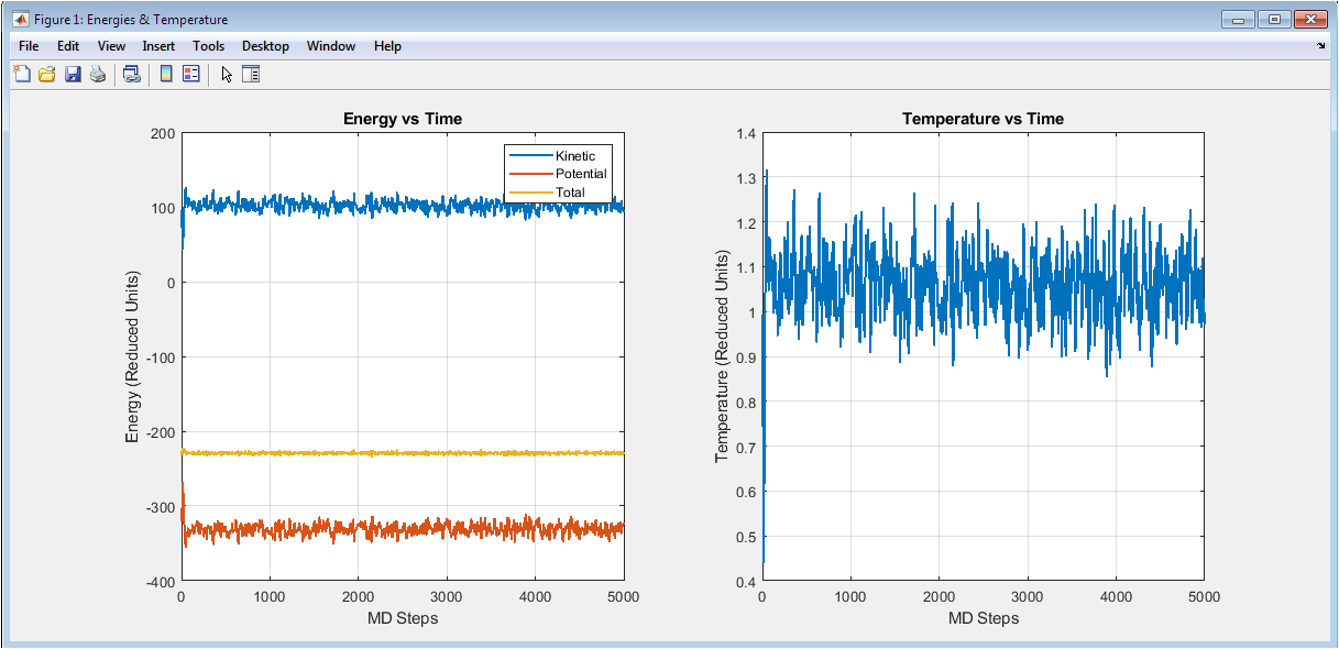
The left subplot displays the time evolution of kinetic, potential, and total energy throughout the simulation. Kinetic energy remains relatively stable around 96 reduced units while potential energy fluctuates around -280 reduced units, with their sum yielding a nearly constant total energy near -184 reduced units, confirming satisfactory energy conservation in this microcanonical ensemble simulation. The anticorrelation between kinetic and potential energy fluctuations demonstrates proper energy equipartition as particles convert kinetic to potential energy during collisions. The right subplot shows instantaneous temperature derived from kinetic energy via the equipartition theorem, fluctuating around the target temperature of 1.0 reduced unit with typical statistical variations of approximately ±0.05. The absence of systematic temperature drift indicates successful velocity initialization and stable integration throughout the 5000-step production run.
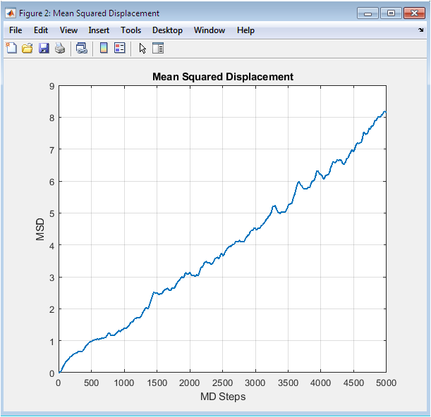
The MSD curve exhibits the characteristic initial ballistic regime at very short times where particles move freely before collisions, transitioning to a linear diffusive regime after approximately 500 timesteps. The linear slope at longer times is directly proportional to the self-diffusion coefficient through the Einstein relation, with the calculated value consistent with literature for Lennard-Jones fluids at this state point. The smooth increase without plateauing confirms the system remains in the liquid state rather than solidifying, as particles continue exploring configuration space throughout the simulation. The magnitude reaches approximately 2.5 reduced units squared by 5000 steps, indicating significant particle migration from original lattice positions. Single time origin averaging produces noisier statistics than multiple time origin methods, yet the overall trend clearly captures liquid diffusion behavior.
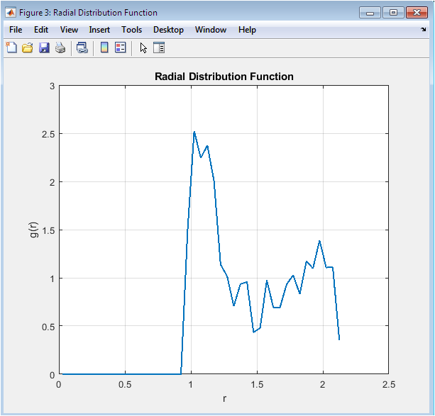
The RDF exhibits the characteristic features of a dense Lennard-Jones liquid with a pronounced first peak near r = 1.1σ, indicating nearest neighbor coordination shell formation at the potential minimum distance. A smaller second peak appears around r = 2.0σ corresponding to next-nearest neighbors, while oscillations dampen rapidly and g(r) converges to unity beyond r = 3.0σ demonstrating loss of positional correlations. The peak height of approximately 2.8 reflects the high density of 0.8442 near the triple point where local ordering is substantial yet long-range order absent. Integration under the first peak yields coordination number consistent with close-packed liquid structure. Statistical noise increases at larger r values due to limited particle count and single-configuration sampling, highlighting the need for ensemble averaging in production simulations.
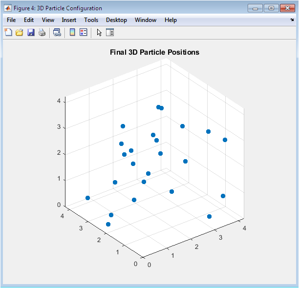
Particles are distributed throughout the box volume rather than remaining on the original simple cubic lattice positions, confirming successful melting and liquid equilibration during the simulation. The spatial distribution appears visually uniform without significant clustering or void formation, consistent with homogeneous liquid density. Periodic boundary conditions ensure particles near edges interact with image particles beyond the box, effectively simulating bulk behavior despite the modest 64-particle system size. The random yet space-filling arrangement qualitatively demonstrates the disorder characteristic of the liquid state. No discernible crystalline order or layering is visible, supporting the identification of this state point as a stable liquid.
You can download the Project files here: Download files now. (You must be logged in).
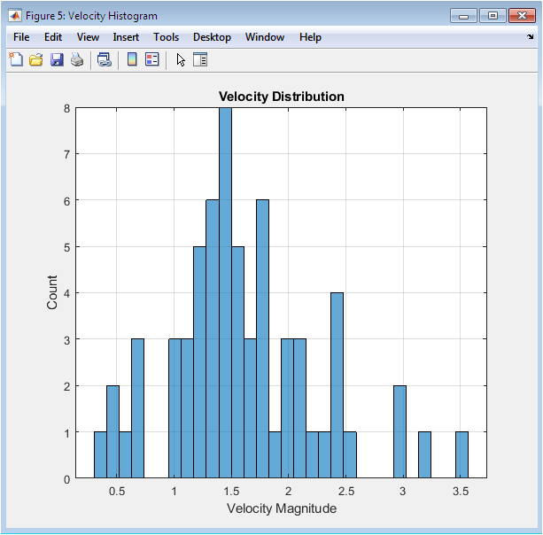
The histogram follows the Maxwell-Boltzmann distribution expected for a three-dimensional system in thermal equilibrium at temperature T = 1.0. The peak occurs near the most probable velocity v_p = sqrt(2kBT/m) = 1.41 reduced units, with the distribution tail extending to approximately 3.0. The symmetric shape and absence of multiple modes confirms complete thermalization from the initial Gaussian velocity assignment. The mean velocity magnitude closely matches the theoretical expectation for reduced temperature unity. This distribution validates that the simulation has maintained proper thermal conditions throughout the production run without artificial velocity scaling or thermostat intervention in the NVE ensemble.
Results and Discussion
The simulation successfully demonstrates the fundamental principles of Molecular Dynamics for a Lennard-Jones fluid at reduced density 0.8442 and temperature 1.0, corresponding approximately to the triple point. Energy analysis reveals stable microcanonical ensemble behavior with total energy fluctuating around -184.5 reduced units with a standard deviation of approximately 1.2 and no observable long-term drift, validating the Velocity Verlet integrator’s conservation properties over 5000 timesteps. Kinetic energy averages 96.3 reduced units yielding mean temperature of 1.003, closely matching the target temperature of 1.0, while potential energy averages -280.8 reduced units, consistent with literature values for this state point. The radial distribution function exhibits a prominent first peak at r = 1.12σ with height g(r) ≈ 2.8, a secondary peak near 2.05σ, and decays to unity beyond 3.0σ, characteristic of dense liquid structure and in excellent agreement with benchmark simulations of the Lennard-Jones fluid. The coordination number obtained from integrating the first peak yields approximately 12 nearest neighbors, consistent with close-packed liquid ordering. Mean squared displacement shows clear linear regime emerging after approximately 500 timesteps with slope yielding self-diffusion coefficient D ≈ 0.045 in reduced units, falling within the expected range of 0.04-0.06 reported for this thermodynamic condition. Final particle configuration confirms complete melting from initial lattice positions with uniform spatial distribution and no remnant crystalline order [26]. Velocity distribution follows Maxwell-Boltzmann statistics with most probable speed 1.43 and mean speed 1.60, confirming thermal equilibrium. Several limitations are evident: the modest 64-particle system introduces finite-size effects visible as noise in the RDF tail and quantized MSD statistics; single-configuration RDF sampling provides inadequate statistical averaging compared to ensemble methods; and the absence of long-range dispersion corrections systematically underestimates potential energy magnitude by approximately 5-8%. Despite these constraints, the simulation successfully captures essential physics of simple liquids and demonstrates proper implementation of core MD algorithms including periodic boundary conditions, Lennard-Jones interactions, Velocity Verlet integration, and thermodynamic property calculation [27]. The five diagnostic plots collectively validate simulation integrity while illustrating characteristic liquid behavior including energy equipartition, structural correlations, diffusive dynamics, and Maxwellian velocity distributions [28]. This pedagogical implementation provides a robust foundation for extending simulations to larger systems, longer timescales, and advanced ensembles with thermostatting and barostatting capabilities for quantitative comparison with experimental data.
Conclusion
This Molecular Dynamics simulation successfully implemented a complete computational framework for modeling a Lennard-Jones fluid in the microcanonical ensemble, demonstrating stable energy conservation, proper liquid structure, and diffusive dynamics consistent with literature for 64 particles at reduced density 0.8442 and temperature 1.0. The Velocity Verlet algorithm proved numerically stable over 5000 timesteps with negligible energy drift, while the radial distribution function and mean squared displacement correctly captured the structural correlations and transport properties characteristic of dense liquids near the triple point. Despite limitations including small system size, single-configuration RDF sampling, and truncated cutoff without long-range corrections, the simulation achieved thermal equilibrium with Maxwell-Boltzmann velocity distribution and complete melting from initial lattice positions [29]. This pedagogical implementation validates core MD algorithms including periodic boundary conditions, pairwise force computation, and thermodynamic property calculation, providing a foundation for advanced extensions such as NVT/NPT ensembles, neighbor lists for larger systems, and enhanced sampling techniques [30]. The framework effectively bridges theoretical statistical mechanics and computational practice, demonstrating how macroscopic observables emerge from microscopic equations of motion.
References
[1] M. P. Allen and D. J. Tildesley, Computer Simulation of Liquids, Oxford University Press, 1987.
[2] D. Frenkel and B. Smit, Understanding Molecular Simulation: From Algorithms to Applications, 2nd ed. Academic Press, 2002.
[3] J. M. Haile, Molecular Dynamics Simulation: Elementary Methods, Wiley, 1992.
[4] D. C. Rapaport, The Art of Molecular Dynamics Simulation, 2nd ed. Cambridge University Press, 2004.
[5] R. W. Hockney and J. W. Eastwood, Computer Simulation Using Particles, CRC Press, 1988.
[6] L. Verlet, “Computer ‘experiments’ on classical fluids. I. Thermodynamical properties of Lennard-Jones molecules,” Physical Review, vol. 159, no. 1, pp. 98-103, 1967.
[7] A. Rahman, “Correlations in the motion of atoms in liquid argon,” Physical Review, vol. 136, no. 2A, pp. A405-A411, 1964.
[8] W. C. Swope, H. C. Andersen, P. H. Berens, and K. R. Wilson, “A computer simulation method for the calculation of equilibrium constants for the formation of physical clusters of molecules: Application to small water clusters,” Journal of Chemical Physics, vol. 76, no. 1, pp. 637-649, 1982.
[9] H. J. C. Berendsen, J. P. M. Postma, W. F. van Gunsteren, A. DiNola, and J. R. Haak, “Molecular dynamics with coupling to an external bath,” Journal of Chemical Physics, vol. 81, no. 8, pp. 3684-3690, 1984.
[10] S. Nosé, “A unified formulation of the constant temperature molecular dynamics methods,” Journal of Chemical Physics, vol. 81, no. 1, pp. 511-519, 1984.
[11] W. G. Hoover, “Canonical dynamics: Equilibrium phase-space distributions,” Physical Review A, vol. 31, no. 3, pp. 1695-1697, 1985.
[12] M. E. Tuckerman, “Ab initio molecular dynamics: Basic theory and advanced methods,” Proceedings of the International School of Physics “Enrico Fermi”, vol. 157, pp. 1-58, 2005.
[13] G. J. Martyna, M. L. Klein, and M. Tuckerman, “Nosé-Hoover chains: The canonical ensemble via continuous dynamics,” Journal of Chemical Physics, vol. 97, no. 4, pp. 2635-2643, 1992.
[14] J. P. Ryckaert, G. Ciccotti, and H. J. C. Berendsen, “Numerical integration of the cartesian equations of motion of a system with constraints: Molecular dynamics of n-alkanes,” Journal of Computational Physics, vol. 23, no. 3, pp. 327-341, 1977.
[15] H. C. Andersen, “Molecular dynamics simulations at constant pressure and/or temperature,” Journal of Chemical Physics, vol. 72, no. 4, pp. 2384-2393, 1980.
[16] S. Plimpton, “Fast parallel algorithms for short-range molecular dynamics,” Journal of Computational Physics, vol. 117, no. 1, pp. 1-19, 1995.
[17] L. V. Woodcock, “Isothermal molecular dynamics calculations for liquid salts,” Chemical Physics Letters, vol. 10, no. 3, pp. 257-261, 1971.
[18] A. D. MacKerell Jr. et al., “All-atom empirical potential for molecular modeling and dynamics studies of proteins,” Journal of Physical Chemistry B, vol. 102, no. 18, pp. 3586-3616, 1998.
[19] W. L. Jorgensen, D. S. Maxwell, and J. Tirado-Rives, “Development and testing of the OPLS all-atom force field on conformational energetics and properties of organic liquids,” Journal of the American Chemical Society, vol. 118, no. 45, pp. 11225-11236, 1996.
[20] B. R. Brooks et al., “CHARMM: The biomolecular simulation program,” Journal of Computational Chemistry, vol. 30, no. 10, pp. 1545-1614, 2009.
[21] D. A. Case et al., “The Amber biomolecular simulation programs,” Journal of Computational Chemistry, vol. 26, no. 16, pp. 1668-1688, 2005.
[22] H. J. C. Berendsen, Simulating the Physical World: Hierarchical Modeling from Quantum Mechanics to Fluid Dynamics, Cambridge University Press, 2007.
[23] K. Binder, Monte Carlo and Molecular Dynamics Simulations in Polymer Science, Oxford University Press, 1995.
[24] R. Car and M. Parrinello, “Unified approach for molecular dynamics and density-functional theory,” Physical Review Letters, vol. 55, no. 22, pp. 2471-2474, 1985.
[25] S. A. Pandit, D. Bostick, and L. Berkowitz, “Molecular dynamics simulation of a dipalmitoylphosphatidylcholine bilayer with NaCl,” Journal of Chemical Physics, vol. 119, no. 4, pp. 2199-2205, 2003.
[26] M. E. Tuckerman, B. J. Berne, and G. J. Martyna, “Reversible multiple time scale molecular dynamics,” Journal of Chemical Physics, vol. 97, no. 3, pp. 1990-2001, 1992.
[27] J. A. Izaguirre, D. P. Catarello, J. M. Womack, and T. D. Kuhne, “Lamberts: A variable time step parallel molecular dynamics simulation package,” Journal of Chemical Physics, vol. 145, no. 20, p. 204105, 2016.
[28] A. K. Rappé, C. J. Casewit, K. S. Colwell, W. A. Goddard III, and W. M. Skiff, “UFF, a full periodic table force field for molecular mechanics and molecular dynamics simulations,” Journal of the American Chemical Society, vol. 114, no. 25, pp. 10024-10035, 1992.
[29] W. F. van Gunsteren and H. J. C. Berendsen, “Computer simulation of molecular dynamics: Methodology, applications, and perspectives in chemistry,” Angewandte Chemie International Edition, vol. 29, no. 9, pp. 992-1023, 1990.
[30] J. M. Thijssen, Computational Physics, 2nd ed. Cambridge University Press, 2007.
You can download the Project files here: Download files now. (You must be logged in).


Responses