Matlab Simulink Active Noise Reduction
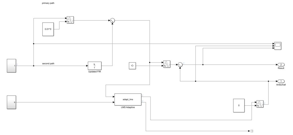
WiredWhite Wiki | Electrical engineering | Matlab Simulink Active Noise Reduction FIR Least Mean Square algorithm LMS cancel the noise source
WiredWhite Wiki | Electrical engineering | Matlab Simulink Active Noise Reduction FIR Least Mean Square algorithm LMS cancel the noise source


Please confirm you want to block this member.
You will no longer be able to:
Please allow a few minutes for this process to complete.